19 Evanescent h

On a radio broadcast, a baseball fanatic described the path of a home run slammed just inside the left-field post: “Coming off the bat, the ball screamed upwards, passing five stories over the head of the first baseman and still gaining altitude. Then, somewhere over mid-left-field, gravity caught up with the ball, forcing it down faster and faster until it crashed into the cheap seats.” A gripping image, perhaps, but wrong about the physics. Gravity does not suddenly catch hold of the ball. Gravity influences the ball in the same way at all phases of flight, upward and downward. The vertical velocity of the ball is positive while climbing and negative on descent, but that velocity is steadily changing all through the flight: a smooth, almost linear numerical decrease in velocity from the time the ball leaves the bat to when it lands in the bleachers.

At each instant, the ball’s vertical velocity has a numerical value in feet-per-second (L T^-1). That value changes continuously. If $Z(t)$ is the height of the ball at time $t$, and $v_Z(t)$ is the vertical velocity at time $t$, then the slope function \[{\cal D}_t Z(t) \equiv \frac{Z(t+h) - Z(t)}{h}\] tells us the average velocity of the ball over a time interval of $h$.

The “average velocity” is a human construction because $h$ is a human choice. The reality pointed to by Newton is that at each instant in time the ball has a continuously changing velocity. Velocity is the physical reality: an instantaneous quantity. The “average velocity” is merely a concession to the way we measure, recording the height at two different times and computing the difference in height divided by the difference in time.

Our average velocity measurement gets closer to the instantaneous velocity when we make the time interval $h$ smaller. But how small?

In the decades after Newton and Leibniz published their work inventing calculus, there was much philosophical concern about $h$. Skeptics pointed out the truth that either $h$ is zero or it is not. If it is zero, then the slope function would be \[{\cal D}_t Z(t) \equiv \frac{Z(t+0) - Z(t)}{0} = \frac{Z(t) - Z(t)}{0} = \frac{0}{0}\ .\] This $0/0$ is not a proper arithmetical quantity. On the other hand, if $h$ is not zero, then the slope function is a human construction involving $h$, not a natural one where $h$ plays no role.

Figure 19.1: The title page of the most famous critique of calculus. The author is George Berkeley.

Newton and Leibniz could not address skeptics except by using suggestive but as yet undefined words. These amount to saying “$h$ vanishes,” or “$h$ is an infinitesimal,” or “$h$ is a nascent quantity.”

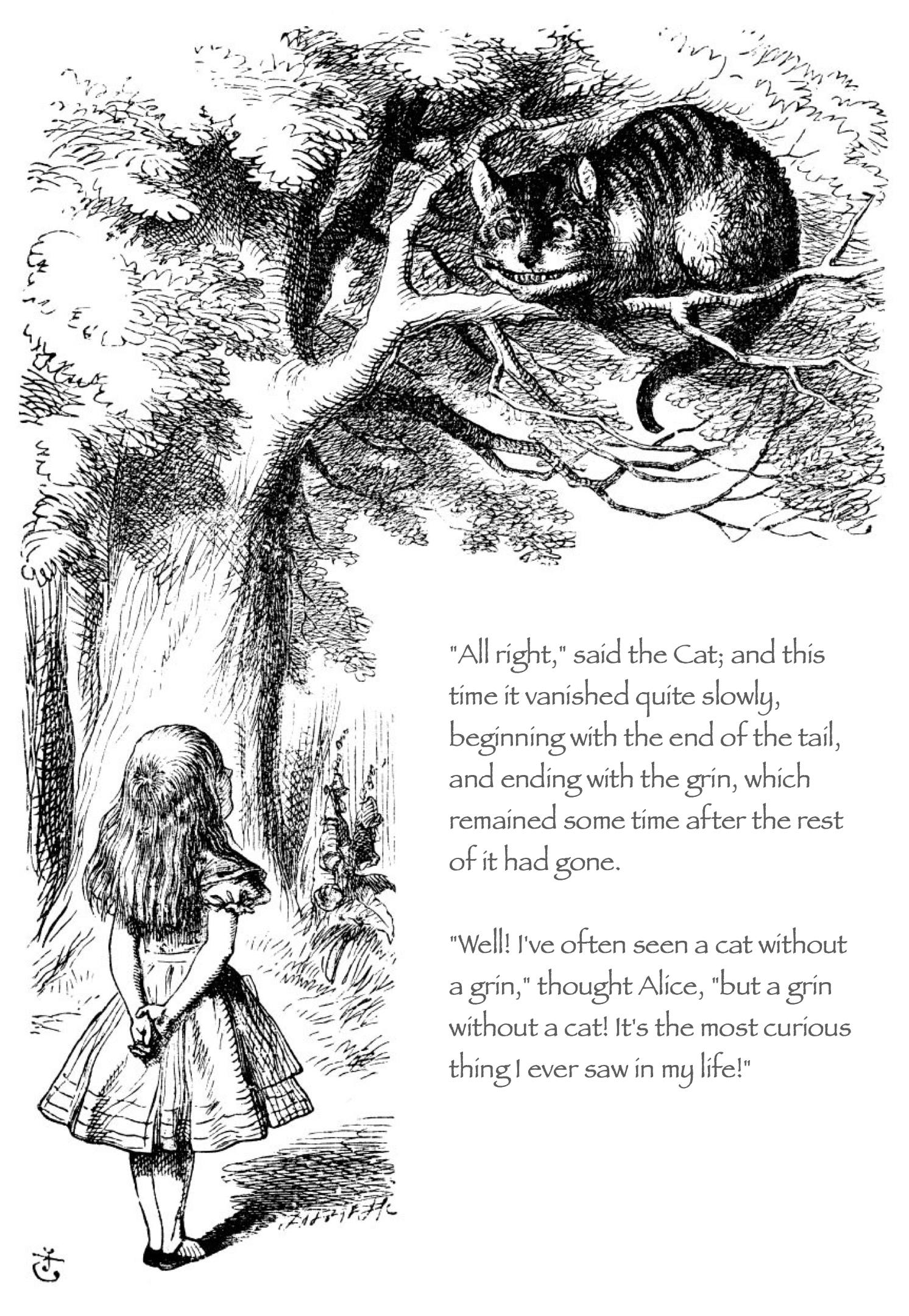
Another good image of $h$ becoming as small as possible comes from University of Oxford mathematician Charles Lutwidge Dodgson (1832-1898). In Alice in Wonderland, Dodgson introduced the character of the Cheshire Cat.

Figure 19.2: Vanishing $h$ in the form of the Chesire Cat from *Alice in Wonderland*.

Math in the World: Ghosts, vapors, and h

The most famous early calculus skeptic, George Berkeley (1685-1753), decried the vanishing $h$ as “notional shadowy Entities.” He described $h$ as “evanescent,” meaning “tending to vanish like vapor.”¹ In Berkeley’s era, the appearance and vanishing of a vapor might well have been a mysterious process. Berkeley used “vapor” as a criticism. He went further:

In 1960 a different rigorous mathematical framework, called non-standard analysis, was introduced. Both theories provide a set of rules for allowed manipulations of algebraic expressions involving $h$: when you can ignore a term involving $h$ and when you cannot. Such rules were used to find the derivatives of basic functions (such as the sinusoid) and to figure out the correct formulas for function products and function composition as in Chapter Chapter 23. Using such formulas does not require re-iterating the historical development of them.

“And what are these same evanescent Increments? They are neither finite Quantities nor Quantities infinitely small, nor yet nothing. May we not call them the ghosts of departed quantities?”

Strangely, Berkeley was not skeptical about the calculations used in calculus. He wrote in The Analysis,² “I have no Controversy about your Conclusions, but only about your Logic and Method….[B]y virtue of a two fold mistake you arrive, though not at science, yet truth.”

Not until 1870 was a rigorous theory of vanishing $h$ accepted by the mathematics community. This theory of limits is sometimes taught as the centerpiece of introductory calculus even though it has little connection to the uses of calculus.

For a physical metaphor for evanescent $h$, consider the process of painting. It is evident that a can of paint contains liquid which somehow becomes solid when brushed on a wall or other object. A better way to think about paint is as a “colloid,” small solid particles suspended in a liquid. The purpose of the liquid is to keep the solid particles separate, so that the paint can flow and conform to the surface of the object being painted. Spreading out the liquid on the surface leads to rapid evaporation so that only the solid particles remain. Without the liquid, the particles no longer flow. They remain in place.

In the expression \[{\cal D}_t p(t) \equiv \frac{p(t+h) - p(t)}{h}\] the quantity $h$ is the liquid and each value of the input is a particle of solid. $h$ separates the solid particles. $p(t+h)$ and $p(t)$ are the values of the function at the slightly separated inputs. Since the inputs are held slightly apart, the function values $p(t+h)$ and $p(t)$ can be distinct and the difference between them, $p(t+h) - p(t)$, can be non-zero. The final result is to remove the $h$ from the difference, that is, divide $p(t+h)-p(t)$ by $h$. By slightly separating the input values, $h$ makes its contribution to the process, but in the end, $h$ evaporates just like the liquid in paint. That is why $h$ is evanescent: eventually it vanishes like vapor.

19.1 Evanescence algebraically

Let’s look at a slope function using evanescent $h$. To start, we will analyze $f(t) \equiv t^2$, one of our pattern-book functions. By definition,

\[{\cal D}_t f(t) \equiv \frac{f(t+h) - f(t)}{h}\ .\]

We can easily evaluate $f(t+h)$ symbolically:

\[f(t+h) \equiv (t+h)^2 = t^2 + 2 t h + h^2\]

Similarly, we can find the difference $f(t+h) - f(t)$. It is

\[f(t+h) - f(t) = f(t+h) - t^2 = 2 t h + h^2\ .\]

Notice that there is still some liquid (that is, $h$) in the difference. Now we let the difference start to dry, taking out the $h$ by dividing the difference by $h$:

\[\frac{f(t+h) - f(t)}{h} = \frac{2 t h + h^2}{h} = 2 t + h\ .\]

The rate of chaange of $f(t)$ has something solid—$2 t$—along with a little bit of liquid $h$ that we can leave to evaporate to nothing.

19.2 Differentiation

By this point you should be familiar with the definition of the average rate of change of $f(t)$ over an interval from $t$ to $t+h$:

\[{\cal D}_t f(t) \equiv \frac{f(t+h) - f(t)}{h}\]

To indicate that we want a rate of change with evanescent $h$, we add a statement to that effect:

\[\partial_t f(t) \equiv \lim_{h\rightarrow 0} {\cal D}_t f(t) = \lim_{h\rightarrow0}\frac{f(t+h) - f(t)}{h}\ .\]

A proper mathematical phrasing of $\lim_{h\rightarrow 0}$ is, “the limit as $h$ goes to zero.” In terms of the paint metaphor, read $\lim_{h\rightarrow 0}$ as “once applied to the wall, let the paint dry.”

To save space, write $\lim_{h\rightarrow 0} {\cal D}_t f(t)$a more compact way: $\partial_t f(t)$. We use the small symbol $\partial$ as a reminiscence of the role that small $h$ played in the construction of $\partial_t f(t)$.

The function $\partial_t f(t)$ is called the derivative of the function $f(t)$. The process of constructing the derivative of a function is called differentiation. The roots of these two words are not the same. “Differentiation” comes from “difference,” a nod to subtraction as in “the difference between 4 and 3 is 1.” In contrast, “derivative” comes from “derive,” whose dictionary definition is “obtain something from a specified source,” as in deriving butter from cream. “Derive” is a general term. But “derivative” and “differentiation” always refers to a specific form of related to rates of change.

19.3 Derivatives of the pattern book functions

The pattern-book functions are so widely used that it is helpful to memorize facts about their derivatives. Remember that, as always, the derivative of a function is another function. For every pattern-book function, the derivative is itself built from a pattern-book functions. To emphasize this, the list below states the rules in terms of the names of the functions, rather than formulas.

$\partial_x$ one(x) $=$ zero(x)
$\partial_x$ identity(x) $=$ one(x)
$\partial_x$ square(x) $=$ 2 identity(x)
$\partial_x$ reciprocal(x) $=$ -1/square(x)
$\partial_x$ log(x) $=$ reciprocal(x)
$\partial_x$ sin(x) $=$ cos(x)
$\partial_x$ exp(x) $=$ exp(x)
$\partial_x$ sigmoid(x) $=$ gaussian(x)
$\partial_x$ gaussian(x) $=$ - x gaussian(x)

In applications, the pattern-book functions are parameterized, e.g. $\sin\left(\frac{2\pi}{P} t\right)$. Chapter 23 introduces the derivatives of the parameterized functions.

Notice that $h$ does not appear at all in the table of derivatives. Instead, to use the derivatives of the pattern-book functions we need only refer to a list of facts, not the process for discovering those facts.

Figure 19.3: A diagram showing how differentiation connects the pattern-book functions to one another.

19.4 Notations for differentiation

There are many notations in wide use for differentiation. In this book, we will denote differentiation in a manner has a close analogy in computer notation.

We will write the derivative of $f(x)$ as $\partial_x f(x)$. If we had a function $g(t)$, with $t$ being the input name, the derivative would be $\partial_t g(t)$. Since there is nothing special about the name of the input in functions with one input, we could just as well write the one-input function that is the derivative of $g()$ with respect to its input as $\partial_x g(x)$ or $\partial_z g(z)$ or even $\partial_{zebra} g(zebra)$. For functions with just one input, the notation skeptic might argue that there is no need for a subscript on $\partial$, since it will always match the name of the input to the function being differentiated.

Early in the history of calculus, mathematician Joseph-Louis Lagrange (1736-1813) proposed a more compact notation for the derivative of a function with a single input. Rather than $\partial_x f(x)$, Lagrange wrote $f'$. We pronounce this “f-prime.” This notation is still widely used in calculus textbooks because it is compact. But it is not a viable notation for functions used in modeling since those functions often have more than one input.

Earlier than Lagrange, Newton used a very compact notation. The historian needs to be careful, because Newton did not use the term “derivative” nor the term “function.” Instead, Newton wrote of “flowing quantities,” that is, quantities that change in time. For Newton, typical names for such flowing quantities were $x$ and $y$. He didn’t use the parentheses that we now associate with functions, just the bare name. Newton used “fluent” to name such flowing quantities. Newton’s fluents were more or less what we call today “functions of time.” What we now call “derivatives,” Newton called “fluxions.” If $x$ is a fluent, then Newton wrote $\dot{x}$ to stand for the fluxion. This is pronounced “x-dot.” Like Lagrange’s compact prime notation, Newton’s dot notation is still used, particularly in physics.

The mathematician Gottfried Wilhelm Leibniz (1646-1716) was a contemporary of Newton. Leibniz developed his own notation for calculus, which was easier to understand than Newton’s. In Leibniz’s notation, the derivative (with respect to $x$) of $f(x)$ was written \[\frac{df}{dx}\ .\] The little $d$ stands for “a little bit of” or “a little change in,” so $\frac{df}{dx}$ makes clear that the derivative is a ratio of two little bits. In the denominator, $dx$ refers to an infinitesimal change in the value of the input $x$. In the numerator, the $df$ names the corresponding change in the output of $f()$ when the input is changed.

Leibniz’s notation is by far the most widely used in introductory calculus. It has many advantages compared to Newton’s or Lagrange’s notations. For example, it provides an opportunity to name the with-respect-to input. It also provides a nice notation for an operation called “anti-differentiation” which we will meet in Part ?sec-accumulation-part. And many a physics or engineering student has been taught to treat $dx$ as if it were a number when doing algebraic manipulations.

The problem with Leibniz’s notation, from the perspective of this book, is that it does not translate well into computer notation. A statement like:

df/dx <- x^2 + 3*x

is a non-starter since the character / is not allowed in a name in most computer languages, including R.

For functions with multiple inputs, for instance, $h(x,y,z)$, differentiation can be done with respect to any input. Leibniz’s notation might possibly be used to indicate which is the with-respect-to input; the three derivatives of $h()$ would be written $dh/dx$ and $dh/dy$ and $dh/dz$. However, mathematical notation did not go in this direction. Instead, for functions with multiple inputs, the three derivatives are most usually written $\partial h/\partial x$ and $\partial h/partial y$, and $\partial h/\partial z$. In the expression, $\partial h/\partial y$, the symbol $\partial$ is pronounced “partial,” The three different derivatives $\partial h/\partial x$, $\partial y /\partial y$, and $\partial h/\partial z$ are called “partial derivatives” and are the subject of Chapter Chapter 25.

This book uses $\partial_x h$, $\partial_y h$, and $\partial_z h$ to denote partial derivatives. This adequately identifies the with-respect-to input and has a close analog in computer notation. For instance, if f(x,y,z) has been defined already, the following statements are entirely valid:

dz_f <- D(f(x,y,z) ~ z)
dy_f <- D(f(x,y,z) ~ y)

It has been more than 300 years since Leibniz’s death. At this point calculus is so we will established that we don’t need the notation $df/dx$ to remind us that a derivative is “a little bit of $f$ divided by a little bit of $x$.”

There are several traditional notations for differentiation of a single-input function named $f()$. Here’s a list of some of them, along with the name associated with each:

Leibnitz: $\frac{df}{dx}$
Partial: $\frac{\partial f}{\partial x}$
Newton (or “dot”): $\dot{f}$
Lagrange (or “prime”): $f'$
One-line (used in this book): $\partial_x f$

To read calculus fluently, you will have to recognize each of these notations. For functions with one input, they all mean the same thing. But when functions have multiple inputs, the choice is between the styles $\partial f / \partial x$ and $\partial_x f$. We use the later because it can easily be incorporated into computer commands.

19.5 Exercises

Exercise 19.02

Let’s explore the derivative $\partial_x \frac{1}{x}$ using the evanescent-h method.

The general definition of the derivative of a function $f(x)$ is the limit as $h\rightarrow 0$ of a ratio:

\[\partial_x f(x) \equiv \underbrace{\lim_{h \rightarrow 0}}_\text{limit}\ \underbrace{\frac{f(x + h) - f(h)}{h}}_\text{ratio}\ .\]

For an evanescent-h calculation, we put aside for a moment $\lim_{h\rightarrow0}$ and operate algebraically on the ratio. In our operations, we treat $h$ as non-zero.

Substitute in $f(x) = 1/x$ and show step-by-step that the ratio (for non-zero $h$) is equivalent to $- \frac{1}{x^2 + hx}$.
The domain of the function $1/x$ is the entire number line, except zero. Examine the expression $- \frac{1}{x^2 + hx}$ to see if setting $h$ to zero would ever involve a division by zero for any $x$ in the domain of $1/x$.
If setting $h=0$ cannot cause a division by zero, it is legitimate to do so. Set $h=0$ and simplify the expression $- \frac{1}{x^2 + hx}$. Compare this to the rule for $\partial_x \frac{1}{x}$ given in Section 19.3.

Exercise 19.03

We don’t yet have the tools needed to prove a formula for the derivative of power-law functions, but we already have some instances where we know the derivative:

$\partial_x x^2 = 2 x$
$\partial_x x^1 = 1$
$\partial_x x^0 = 0$

A rule that fits all these examples is \[\partial_x x^p = p\, x^{p-1}\ .\] For instance, when $p=2$ the rule gives \[\partial_x x^2 = 2\, x^1 = 2 x\] since $p-1$ will be 1$.

It is not too hard to do the algebra to find the derivative of $x^3$. According to the proposed rule, the derivative should be \[\partial_x x^3 = 3 x^2\ .\]

Let’s check this via the general definition of the derivative:

\[\partial_x x^3 = \underbrace{\lim_{h \rightarrow 0}}_\text{limit}\ \underbrace{\frac{(x+h)^3 - x^3}{h}}_\text{ratio}\]

In the evanescent-h technique, we put aside the limit for a moment and work algebraically on the ratio with the assumption that $h\neq0$.

Expand out $(x+h)(x+h)(x+h) - x^3$ to get a linear combination of monomials: $x^2$, $x^1$, and $x^0$.

Divide the linear combination in (a) by $h$ and simplify.
Examine the expression from (b) to determine if setting $h=0$ will result in a divide-by-zero. What did you find?
If your conclusion from (c) is that divide-by-zero does not occur when $h=0$, set $h=0$ and simplify the expression from (b) to find $\partial_x x^3$. Is your result consistent with the rule for the derivative of power-law functions described at the beginning of this problem.

Problem with Differentiation Differentiation/Exercises/shark-tug-laundry.Rmd

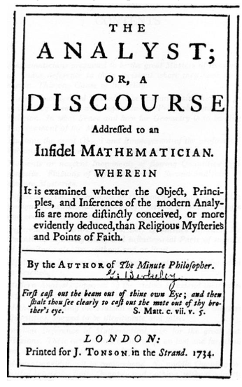
https://www.merriam-webster.com/dictionary/evanescent ↩︎
Full title: The Analyst: A Discourse Addressed to an Infidel Mathematician: Wherein It Is Examined Whether the Object, Principles, and Inferences of the Modern Analysis Are More Distinctly Conceived, or More Evidently Deduced, Than Religious Mysteries and Points of Faith↩︎