install.packages("mosaicCalc")3 Computing with R
Mathematical notation evolved for the purpose of communication among people. With the introduction of programmable computers in the middle of the 20th century, a notation was needed to communicate between people and hardware. It turns out that traditional mathematical notation in calculus is not fully adequate for this purpose. This chapter introduces the notation used in R/mosaic.
3.1 Commands and evaluation
Computers need to distinguish between declarative and imperative statements. A declarative statement, like \(g(z) \equiv z \cos(z)\) defines and describes a relationship. An imperative statement is a direction to do some action. For instance, “The store is on the next block,” is declarative. “Bring some crackers from the store,” is imperative. Evaluating a function calls for an imperative statement.
\(\equiv\) and \(=\) are declarative
Noting the distinction between declarative and imperative helps to better understand mathematical notation. In a mathematical statement like \(h(x) \equiv 3 x + 2\), the \(\equiv\) indicates that the statement is declarative. Similarly, the equal sign is used for declarative statements, as with \[\pi = 3.14159\ldots\] On the other hand, applying a function to a value, as in \(h(3)\), is an imperative statement.
The names and format of such instructions—e.g. make a mathematical function from a formula, draw a graph of a function, plot data—are given in the same name/parentheses notation we use in math. For example, makeFun() constructs a function from a formula, slice_plot() graphs a function, gf_point() makes one style of data graphic. These R entities saying “do this” are also called “functions.”
When referring to such R “do this” functions, we will refer to the stuff that goes in between the parentheses as “arguments.” The word “input” would also be fine. The point of using “input” for math functions and “argument” for R “do-this” functions is merely to help you identify when we are talking about mathematics and when we are talking about computing.
With computers, writing an expression in computer notation goes hand-in-hand with evaluating the notation. In the mode we will use in this book, you enter your commands in an editor block that we call an “active R chunk.” An example is Active R chunk lst-very-first-one, where the editor has been pre-populated with a simple arithmetic command: 2 + 3.
To evaluate the command, press the “Run Code” button. You can edit the command in the usual way, placing the cursor in the editor block and typing.
In Active R chunk lst-very-first-one (as it initially appears) there is a 1 at the far left. This is a line number, not part of a command. Active R chunks can contain multiple lines and even multiple commands.
Important 3.1: Simple editing
Modify the contents of Active R chunk lst-very-first-one to subtract 22 from 108. Confirm that running the code produces an output of 86.
The R language is set up to format the printing of returned values with an index, which is helpful when the value of the expressions is a large set of numbers. In the case here, with just a single number in the result of evaluating the expression, the index is simply stating the obvious.
Important 3.2: “Calling” a function
Leaving the command from Try it! try-very-first-one in place, add a second line to Active R chunk lst-very-first-one to calculate \(\sqrt{17}\). (In R, the square-root function is named sqrt().) When you run the code, you will see two outputs: one for the first line and the other for the second line.
Strictly speaking, we can say that running the code sqrt(17) is invoking the function sqrt() on the input value 17. It’s very common in the world of computing to use the word “calling” rather than “invoking.” So, in Try it! try-sqrt-17 you have “called sqrt().
An important form of R expression is storage, a declarative statement. Storage uses a symbolic name and the <- token. Active R chunk lst-assignment-1 gives a simple example using the name b.
We call <- the “storage arrow.” Think of it as stowing the left-hand value in a box labelled with the name on the right-hand side. When storing a value, R is designed not to display the value as happened in the imperative statements in Try it try-very-first-one and [-try-sqrt-17].
Important 3.3: Accessing stored values by name
The purpose of storage is to provide access to a value later on. In order to retrieve the value stored under a name, simply give the name as a command, as in Active R chunk lst-retrieve-b.
Some students may have gotten a response from Active R chunk lst-retrieve-b in the form of an “error message” such as Error: object ‘b’ not found. Even experts get such error messages; it’s easy to make a mistake when forming a computer command. It’s important for newbies to understand that error messages are intended to help you fix things rather than to frighten you. Perhaps being gentler would help here—Sorry, but the object ‘b’ wasn’t found.—but “errors” are part of computing culture.
The message “object ‘b’ not found” is an indication that nothing has yet been stored under the name b. This would be the case if you had neglected to run the code in Active R chunk lst-assignment-1. If that’s your situation, go back to Active R chunk lst-assignment-1 and run the code, then try Active R chunk lst-retrieve-b again.
Within a document, for instance a chapter of this book or from the MOSAIC Calculus Workbook all the active R chunks have access to the work of the other chunks in the document. Understandably, you need to run the code in a chunk in order for other chunks to access it.
Whenever you refresh or re-open a document, the active R chunks will all in a not-yet-run state. You have to run the code individually for each chunk you want to use or which are used by other chunks. By and large, we write each R chunks to avoid the need to run earlier chunks … but not always!
Using R as a stand-alone app
Professionals are used to R coming in the form of a stand-alone app. The most popular such app is RStudio, available as free, open-source software produced by a public benefit corporation, Posit PBC.
There are many tutorials on installing and using RStudio. People do this especially when they need to document and preserve their work or integrate computing into documents. (This book is an example of such a document.) MOSAIC Calculus is written so that you do not need to use anything but the active R chunks. Still, you might prefer to use the many helpful features that RStudio adds to work with the R language. (Advantages of the active R chunks: the student doesn’t need to install any software. It’s nice as well to be able to refer to computations by pointing to a specific active R chunk like Active R chunk lst-very-first-one.)
If you do use RStudio, note that in addition to the app, you need to install several packages from the R ecosystem. You do this from within R. The following R command will do the job:
Then, each time you open RStudio, you need to tell R that you are planning to use the {mosaicCalc} package. Do this as follows:
library(mosaicCalc)3.2 Defining mathematical functions in R/mosaic
As you progress through this book you will meet a dozen or so functions from R/mosaic. For instance, sec-graphs-and-graphics introduces functions for drawing graphs. sec-data-and-data-graphics shows how to plot data.
In this section, we introduce the R/mosaic function for creating mathematical functions.
As you know, our mathematical notation for defining a function looks like this: \[h(t) \equiv 1.5\, t^2 - 2\ .\]
The R/mosaic equivalent to this is
Laying out the two notation forms side by side lets us label the elements they share:
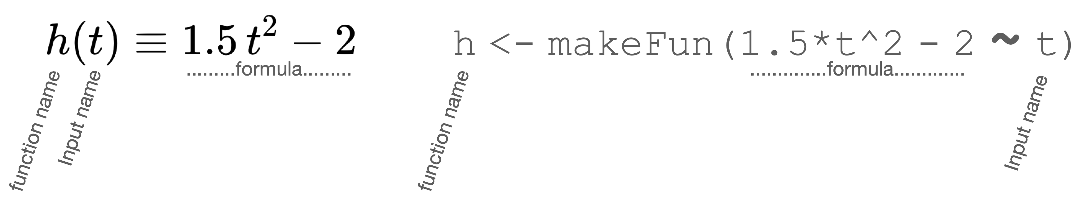
For the human reading the mathematical notation, you know that the statement defines a function because you have been taught so. Likewise, the computer needs to be told what to do with the provided information. That is the point of makeFun(). There are other R/mosaic commands that could take the same information and do something else with it, for example create a graph of the function or (for those who have had some calculus) create the derivative or the anti-derivative of the function.
At its simplest, makeFun() takes only one argument. That argument must be in a form called a tilde expression. This name comes from the character tilde (~) in the middle. On the right-hand side of the tilde goes the name of the input: ~ t. On the left-hand side is the R expression for the formula to be used. The formula is written using the input name and whatever parameters are used. For instance, Active R chunk lst-h-with-params defines a parameterized version of \(h()\).
In Active R chunk lst-h-with-params, three arguments are being provided:
- The tilde expression
a*t^2 - b ~ t - A default value for parameter
a. - A default value for parameter
b.
Important 3.4: Evaluating
h() at an input.
In Active R chunk lst-h-with-params2, write each of the following commands.
- Evaluate
h()for the input \(t = 1\). - Evaluate
h()for the input \(t = 2\). - Repeat (i) and (ii), but override the default value of
b, setting it instead to be \(b=100\).
Naturally, you need to run the code in Active R chunk lst-h-with-params before you can evaluate h().
3.3 Names and assignment
The command
h <- makeFun(1.5*t^2 - 2 ~ t)gives the name h to the function created by makeFun(). Good choice of names makes your commands much easier for the human reader.
Valid and invalid names in R
The R language puts some restrictions on the names that are allowed. Keep these in mind as you create R names in your future work:
- A name is the only thing allowed on the left side of the storage arrow
<-. (For experts … there are additional allowed forms for the left-hand side. We will not need them in this book.) - A name must begin with a letter of the alphabet, e.g.
able,Baker, and so on. - Numerals can be used after the initial letter, as in
final4org20. You can also use the period.and underscore_as inthird_place. No other characters can be used in names: no minus sign, no@sign, no/or+, no quotation marks, and so on.
For instance, while third_place is a perfectly legitimate name in R, the following are not: 3rd_place, third-place. But it is OK to have names like place_3rd or place3, etc., which start with a letter.
R also distinguishes between letter case. For example, Henry is a different name than henry, even though they look the same to a human reader.
3.4 Formulas in R
The constraint of the keyboard means that computer formulas are written in a slightly different way than the traditional mathematical notation. This is most evident when writing multiplication and exponentiation. Multiplication must always be indicated with the * symbol, for instance \(3 \pi\) is written 3*pi. For exponentiation, instead of using superscripts like \(2^3\) you use the “caret” character, as in 2^3. The best way to learn to implement mathematical formulas in a computer language is to read examples and practice writing them. Several examples are given in Table tbl-parallel-commands.
| Traditional notation | R notation |
|---|---|
| \(3 + 2\) | 3 + 2 |
| \(3 \div 2\) | 3 / 2 |
| \(6 \times 4\) | 6 * 4 |
| \(\sqrt{\strut4}\) | sqrt(4) |
| \(\ln 5\) | log(5) |
| \(2 \pi\) | 2 * pi |
| \(\frac{1}{2} 17\) | (1 / 2) * 17 |
| \(17 - 5 \div 2\) | 17 - 5 / 2 |
| \(\frac{17 - 5}{\strut 2}\) | (17 - 5) / 2 |
| \(3^2\) | 3^2 |
| \(e^{-2}\) | exp(-2) |