36 Integration

Anti-derivatives are useful when you know how a quantity is changing but don’t yet know the quantity itself.

It is important, of course, to keep track of which is the “quantity itself” and which is the “rate of increase in that quantity.” This always depends on context and your point of view. It is convenient, then, to set some fixed examples to make it easy to keep track of which quantity is which.

Context	Quantity	Rate of increase in quantity
Money	Cash on hand ${\mathbf S}(t)$	Cash flow $s(t)$
Fuel	Amount in fuel tank ${\mathbf F}(t)$	Fuel consumption rate, e.g. kg/hour $f(t)$
Motion	Momentum ${\mathbf M}(t)$	Force $m(t)$
notation	${\mathbf H}(t)$	$\partial_t {\mathbf H}(t)$
notation	$G(t) = \int g(t) dt$	$g(t)$

We will also adopt a convention to make it simpler to recognize which quantity is the “quantity itself” and which is the “rate of increase in that quantity.” We will use CAPITAL LETTERS to name functions that are the quantity itself, and lower-case letters for the rate of increase in that quantity. For example, if talking about motion, an important quantity is momentum and how it changes over time. The momentum itself will be ${\mathbf M}(t)$ while the rate of increase of momentum will be $m(t)$.¹ The amount of money a business has on hand at time $t$ is ${\mathbf S}(t)$ measured, say, in dollars. The rate of increase of that money is $s(t)$, in, say, dollars per day.

Notice that we are using the phrase “rate of increase” rather than “rate of change.” that is because we want to keep straight the meaning of the sign of the lower-case function. If $m(t)$ is positive, the momentum is increasing. If $m(t)$ is negative then it is a “negative rate of increase,” which is, of course, just a “decrease.”

For a business, money coming in means that $s(t)$ is positive. Expenditures of money correspond to $s(t)$ being negative. In the fuel example. ${\mathbf F}(t)$ is the amount of fuel in the tank. $f(t)$ is the rate of increase in the amount of fuel in the tank. Of course, engines burn fuel, removing it from the tank. So we would write the rate at which fuel is burned as $-f(t)$: removing fuel is a negative increase in the amount of fuel, an expenditure of fuel.

The objective of this chapter is to introduce you to the sorts of calculations, and their notations, that let you figure out how much the CAPITAL LETTER quantity has changed over an interval of $t$ based on what you already know about the value over time of the lower-case function.

The first step in any such calculation is to find or construct the lower-case function $f(t)$ or $c(t)$ or $m(t)$ or whatever it might be. This is a modeling phase. In this chapter, we will ignore detailed modeling of the situation and just present you with the lower-case function.

The second step in any such calculation is to compute the anti-derivative of the lower-case function, giving as a result the CAPITAL LETTER function. You’ve already seen the notation for this, e.g.

\[{\Large F(t) = \int f(t) dt}\ \ \ \ \ \text{or}\ \ \ \ \ {\Large G(t) = \int g(t) dt}\ \ \ \ \text{and so on.}\] In this chapter, we will not spend any time on this step; we will assume that you already have at hand the means to compute the anti-derivative. (Indeed, you already have antiD() available which will do the job for you.) Later chapters will look at the issues around and techniques for doing the computations by other means.

The remaining steps in such calculations are to work with the CAPITAL LETTER function to compute such things as the amount of that quantity, or the change in that quantity as it is accumulated over an interval of $t$.

Why capital letters?

Sometimes we write capital letter functions in bold-face, e.g. ${\mathbf F}(t)$ and other times you aren’t, e.g. $F(t)$. What’s going on?

This is a convention we are adopting for this chapter, which is when we need it the most to introduce the concepts.

Bold-face is being used in this chapter to represent the real-world quantity of interest. So ${\mathbf F}(t)$ is the actual amount of fuel in the tank, ${\mathbf M}(t)$ is the actual momentum of the car, and ${\mathbf S}(t)$ is the actual amount of money on hand. The regular-face functions, $F(t)$ and $M(t)$ and $S(t)$ are the functions that we get by applying anti-differentiation to $f(t)$ or $m(t)$ or $s(t)$.

Our broad interest is to construct the bold-face function knowing just the derivative of that function, which we are writing in lower-case. So, $f(t) \equiv \partial_t {\mathbf F}(t)$. Similarly, $m(t) \equiv \partial_t {\mathbf M}(t)$ and $s(t) \equiv \partial_t {\mathbf S}(t)$. We are in the situation where we know $f(t)$ but not ${\mathbf F}(t)$, or we know $m(t)$ but not ${\mathbf M}(t)$, and so on.

How could such a situation arise in the real world? Suppose the car’s fuel gauge is broken, leaving us without direct knowledge of $\mathbf F$ (liters). But there is a dashboard readout of the instantaneous rate of fuel consumption (say, liters per 100 km). So, we know $f(t)$ but not ${\mathbf F}(t)$. Or suppose you are in charge of day-to-day running of a business, collecting the income each day and paying the daily expenses. Thus, each day you know $s(t)$—the cash flow. But it is your boss who has access to the bank account; you merely deposit money as you get it and authorize electronic funds transfers to suppliers. Your boss knows ${\mathbf S}(t)$ but you know only $s(t)$.

Anti-differentiation is part of the way to reconstruct the fuel level ${\mathbf F}(t)$ from the known $f(t)$, or to figure out the bank balance ${\mathbf S}(t)$ from your records of $s(t)$.

But anti-differentiation, while part of the solution, is only just a part. You can apply anti-differentiation to $f(t)$, but what you get back will be $F(t)$, not ${\mathbf F}(t)$.

What’s the difference between the two? It involves a constant value $C$ which, alas, you can never figure out from $f(t)$. All that you can claim, given the $F(t)$ generated by anti-differentiation, is that \[{\mathbf F}(t) = F(t) + C .\]

36.1 Net change

Perhaps it goes without saying, but once you have the CAPITAL LETTER function, e.g. $F(t)$, you can evaluate that function at any input that falls into the domain of $F(t)$. If you have a graph of $F(t)$ versus $t$, just position your finger on the horizontal axis at input $t_1$, then trace up to the function graph, then horizontally to the vertical axis where you can read off the value $F(t_1)$. If you have $F()$ in the form of a computer function, just apply $F()$ to the input $t_1$.

In this regard, $F(t)$ is like any other function.

However, in using and interpreting the $F(t)$ that we constructed by anti-differentiating $f(t)$, we have to keep in mind the limitations of the anti-differentiation process. In particular, any function $f(t)$ does not have a unique anti-derivative function. If we have one anti-derivative, we can always construct another by adding some constant: $F(t) + C$ is also an anti-derivative of $f(t)$.

But we have a special purpose in mind when calculating $F(t_1)$. We want to figure out from $F(t)$ how much of the quantity $f(t)$ has accumulated up to time $t_1$. For example, if $f(t)$ is the rate of increase in fuel (that is, the negative of fuel consumption), we want $F(t_1)$ to be the amount of fuel in our tank at time $t_1$. That cannot happen. All we can say is that $F(t_1)$ is the amount of fuel in the tank at $t_1$ give or take some unknown constant C.

Instead, the correct use of $F(t)$ is to say how much the quantity has changed over some interval of time, $t_0 \leq t \leq t_1$. This “change in the quantity” is called the net change in $F()$. To calculate the net change in $F()$ from $t_0$ to $t_1$ we apply $F()$ to both $t_0$ and $t_1$, then subtract:

\[\text{Net change in}\ F(t) \ \text{from}\ t_0 \ \text{to}\ t_1 :\\= F(t_1) - F(t_0)\]

Suppose you have already constructed the rate-of-change function for momentum $m()$ and implemented it as an R function m(). For instance, $m(t)$ might be the amount of force at any instant $t$ of a car, and ${\mathbf M}(t)$ is the accumulated force, better known as momentum. We will assume that the input to m() is in seconds, and the output is in kg-meters-per-second-squared, which has the correct dimension for force.

You want to find the amount of force accumulated between time $t=2$ and $t=5$ seconds.

# You've previous constructed m(t)
M <- antiD(m(t) ~ t)
M(5) - M(2)
## [1] -1.392131

To make use of this quantity, you will need to know its dimension and units. For this example, where the dimension [$m(t)$] is M L T$^{-2}$, and [$t$] = T, the dimension [${\mathbf M}(t)$] will be M L T$^{-1}$. In other words, if the output of $m(t)$ is kg-meters-per-second-squared, then the output of $V(t)$ must be kg- meters-per-second.

36.2 The “definite” integral

We have described the process of calculating a net change from the lower-case function $f(t)$ in terms of two steps:

Construct $F(t) = \int f(t) dt$.
Evaluate $F(t)$ at two inputs, e.g. $F(t_2) - F(t_1)$, giving a net change, which we will write as ${\cal F}(t_1, t_2) = F(t_2) - F(t_1)$.

As a matter of notation, the process of going from $f(t)$ to the net change is written as one statement.

\[{\cal F}(t_1, t_2) = F(t_2) - F(t_1) = \int_{t_1}^{t_2} f(t) dt\]

The punctuation \[\int_{t_1}^{t_2} \_\_\_\_ dt\] captures in one construction both the anti-differentiation step ($\int\_\_dt$) and the evaluation of the anti-derivative at the two bound $t_2$ and $t_1$.

Several names are used to describe the overall process. It is important to become familiar with these.

$\int_a^b f(t) dt$ is called a definite integral of $f(t)$.
$a$ and $b$ are called, respectively, the lower bound of integration and the upper bound of integration, although given the way we draw graphs it might be better to call them the “left” and “right” bounds, rather than lower and upper.
The pair $a, b$ is called the bounds of integration.

As always, it pays to know what kind of thing is ${\cal F}(t_1, t_2)$. Assuming that $t_1$ and $t_2$ are fixed quantities, say $t_1 = 2$ seconds and $t_2 = 5$ seconds, then ${\cal F}(t_1, t_2)$ is itself a quantity. The dimension of that quantity is [$F(t)$] which in turn is [$f(t)$]$\cdot$[$t$]. So if $f(t)$ is fuel consumption in liters per second, then $F(t)$ will have units of liters, and ${\cal F}(t_1, t_2)$ will also have units of liters.

Remember also an important distinction:

$F(t) = \int f(t) dt$ is a function whose output is a quantity.
$F(t_2) - F(t_1) = \int_{t_1}^{t_2} f(t) dt$ is a quantity, not a function.

Of course, $f(t)$ is a function whose output is a quantity. In general, the two functions $F(t)$ and $f(t)$ produce outputs that are different kinds of quantities. For instance, the output of $F(t)$ is liters of fuel while the output of $f(t)$ is liters per second: fuel consumption. Similarly, the output of $S(t)$ is dollars, while the output of $s(t)$ is dollars per day.

The use of the term definite integral suggests that there might be something called an indefinite integral, and indeed there is. “Indefinite integral” is just a synonym for “anti-derivative.” In this book we favor the use of anti-derivative because it is too easy to leave off the “indefinite” and confuse an indefinite integral with a definite integral. Also, “anti-derivative” makes it completely clear what is the relationship to “derivative.”

Since 1700, it is common for calculus courses to be organized into two divisions:

Differential calculus, which is the study of derivatives and their uses.
Integral calculus, which is the study of anti-derivatives and their uses.

Mathematical notation having been developed for experts rather than for students, very small typographical changes are often used to signal very large changes in meaning. When it comes to anti-differentiation, there are two poles of fixed meaning and then small changes which modify the meaning. The poles are:

Anti-derivative: $\int f(t) dt$, which is a function whose output is a quantity.
Definite integral $\int_a^b f(t) dt$, which is a quantity, plain and simple.

But you will also see some intermediate forms:

$\int_a^t f(t) dt$, which is a function with input $t$.
$\int_a^x f(t) dt$, which is the same function as in (a) but with the input name $x$ being used.
$\int_t^b f(t) dt$, which is a function with input $t$.
Less commonly, $\int_x^t f(t) dt$ which is a function with two inputs, $x$ and $t$. The same is true of $\int_x^y f(t) dt$ and similar variations.

36.3 Initial value of the quantity

Recall that we are interested in a real quantity ${\mathbf F}(t)$, but we only know $f(t)$ and from that can calculate an anti-derivative $F(t)$. The relationship between them is \[{\mathbf F}(t) = F(t) + C\] where $C$ is some fixed quantity that we cannot determine directly from $f(t)$.

Still, even if we cannot determine $C$, there is one way we can use $F(t)$ to make definite statements about ${\mathbf F}(t)$. Consider the net change from $t_1$ to $t_2$ in the real quantity ${\mathbf F}$. This is

\[{\mathbf F}(t_2) - {\mathbf F}(t_1) = \left[F(t_2) + C\right] - \left[F(t_1) + C\right] = F(t_2) - F(t_1)\]

In other words, just knowing $F(t)$, we can make completely accurate statements about net changes in the value of ${\mathbf F}(t)$.

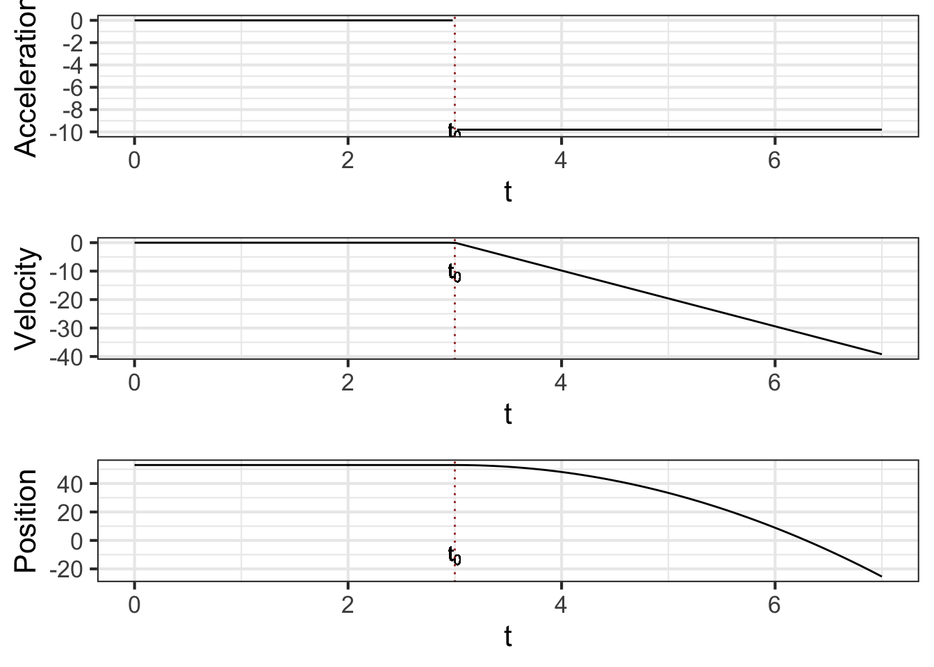
Let’s develop our understanding of this unknown constant $C$, which is called the constant of integration. To do so, watch the movie in Figure 36.1 showing the process of constructing the anti-derivative \[F(t) = \int_2^t f(t) dt\ .\]

Figure 36.1: Constructing the anti-derivative $F(t)$ by reading the slope from $f(t)$ and using that slope to extend the picture of $F()$

Focus first on the top graph. The function we are integrating, $f(t)$, is known before we carry out the integration, so it is shown in the top graph.

$f(t)$ is the rate of increase in $F(t)$ (or ${\mathbf F}(t)$ for that matter). From the graph, you can read using the vertical axis the value of $f(t)$ for any input $t$. But since $f(t)$ is a rate of increase, we can also depict $f(t)$ as a slope. That slope is being drawn as a $\color{magenta}{\text{magenta}}$ arrow. Notice that when $f(t)$ is positive, the arrow slopes upward and when $f(t)$ is negative, the arrow slopes downward. The steepness of the arrow is the value of $f(t)$, so for inputs where the value of $f(t)$ is far from zero the arrow is steeper than for values of $f(t)$ that are near zero.

Now look at both graphs, but concentrate just on the arrows in the two graphs. They are always the same: carbon copies of one another.
Finally the bottom graph. We are starting the integral at $t_1=2$. Since nothing has yet been accumulated, the value $F(t_1 = 2) = 0$. From (1) and (2), you know the arrow shows the slope of $F(t)$. So as $F(t>2)$ is being constructed the arrow guides the way. When the slope arrow is positive, $F(t)$ is growing. When the slope arrow is negative, $F(t)$ is going down.

In tallying up the accumulation of $f(t)$, we started at time $t=2$ and with $F(t=2) = 0$. This makes sense, since nothing can be accumulated over the mere instant of time from $t=2$ to $t=2$. On the other hand, it was our choice to start at $t=2$. We might have started at another value of $t$ such as $t=0$ or $t=-5$ or $t=-\infty$. If so, then the accumulation of $f(t)$ up to $t=2$ would likely have been something other than zero.

But what if we knew an actual value for ${\mathbf F}(2)$. This is often the case. For instance, before taking a trip you might have filled up the fuel tank. The accumulation of fuel consumption only tells you how much fuel has been used since the start of the trip. But if you know the starting amount of fuel, by adding that to the accumulation you will know instant by instant how much fuel is in the tank. In other words, \[{\mathbf F}(t) = {\mathbf F}(2) + \int_2^t f(t) dt\ .\] This is why, when we write an anti-derivative, we should always include mention of some constant $C$—the so-called constant of integration—to remind us that there is a difference between the $F(t)$ we get from anti-differentiation and the ${\mathbf F}(t)$ of the function we are trying to reconstruct. That is,

\[{\mathbf F}(t) = F(t) + C = \int f(t) dt + C\ .\]

We only need to know ${\mathbf F}(t)$ at one point in time, say $t=0$, to be able to figure out the value of $C$: \[C = {\mathbf F}(0) - F(0)\ .\]

Another way to state the relationship between the anti-derivative and ${\mathbf F}(t)$ is by using the anti-derivative to accumulate $f(t)$ from some starting point $t_0$ to time $t$. That is:

\[{\mathbf F}(t) \ =\ {\mathbf F}(t_0) + \int_{t_0}^t f(t)\, dt\ = \ {\mathbf F}(t_0) + \left({\large\strut}F(t) - F(t_0)\right)\]

Math in the World: Galileo in Pisa

An oft-told legend has Galileo at the top of the Tower of Pisa around 1590. The legend illustrates Galileo’s finding that a light object (e.g. a marble) and a heavy object (e.g. a ball) will fall at the same speed. Galileo published his mathematical findings in 1638 in Discorsi e Dimostrazioni Matematiche, intorno a due nuove scienze. (English: Discourses and Mathematical Demonstrations Relating to Two New Sciences)

In 1687, Newton published his world-changingPhilosophiae Naturalis Principia Mathematica. (English: Mathematical Principles of Natural Philosophy)

Let’s imagine the ghost of Galileo returned to Pisa in 1690 after reading Newton’s Principia Mathematica. In this new legend, Galileo holds a ball still in his hand, releases it, and figures out the position of the ball as a function of time.

Although Newton famously demonstrated that gravitational attraction is a function of the distance between to objects, he also knew that at a fixed distance—the surface of the Earth—gravitational acceleration was constant. So Galileo was vindicated by Newton. But, although gravitational acceleration is constant from top to bottom of the Tower of Pisa, Galileo’s ball was part of a more complex system: a hand holding the ball still until release. Acceleration of the ball versus time is therefore approximately a Heaviside function:

$\text{accel}(t) \equiv \left\{\begin{array}{rl}0 & \text{for}\ t \leq 3\\ {-9.8} & \text{otherwise}\end{array}\right.$

accel <- makeFun(ifelse(t <= 3, 0, -9.8) ~ t)

Acceleration is the derivative of velocity. We can construct a function $V(t)$ as the anti-derivative of acceleration, but the real-world velocity function will be

\[{\mathbf V}(t) = {\mathbf V}(0) + \int_0^t \text{accel}(t) dt\]

V_from_antiD <- antiD(accel(t) ~ t)
V <- makeFun(V0 + (V_from_antiD(t) - V_from_antiD(0)) ~ t, V0 = 0)

In the computer expression, the parameter V0 stands for ${\mathbf V}(0)$. We’ve set it equal to zero since, at time $t=0$, Galileo was holding the ball still.

Velocity is the derivative of position, but the real-world velocity function will be the accumulation of velocity from some starting time to time $t$, plus the position at that starting time:

\[x(t) \equiv x(0) + \int_0^t V(t) dt\]

We can calculate $\int V(t) dt$ easily enough with antiD(), but the function $x(t)$ involves evaluating that anti-derivative at times 0 and $t$:

x_from_antiD <- antiD(V(t) ~ t)
x <- makeFun(x0 + (x_from_antiD(t) - x_from_antiD(0)) ~ t, x0 = 53)

We’ve set the parameter x0 to be 53 meters, the height above the ground of the top balcony on which Galileo was standing for the experiment.

Figure 36.2: The acceleration, velocity, and position of the ball as a function of time in Galileo’s Tower of Pisa experiment. The ball is released at time $t_0$.

In the (fictional) account of the 1690 experiment, we had Galileo release the ball at time $t=0$. That is a common device in mathematical derivations, but in a physical sense it is entirely arbitrary. Galileo might have let go of the ball at any other time, say, $t=3$ or $t=14:32:05$.

A remarkable feature of integrals is that it does not matter what we use as the lower bound of integration, so long as we set the initial value to correspond to that bound.

Why $\int f(x) dx$ instead of $\int f(t) dt$?

For a while you were writing integrals like this: $\int_a^b f(t) dt$. Then you replaced $b$ with the input name $t$ to get $\int_a^t f(t) dt$. But then you switched everything up by writing $\int_a^t f(x) dx$. Is that the same as $\int_a^t f(t) dt$? If so, why do you get to replace the $t$ with $x$ in some places but not in others?

Recall from Chapter 2 that the names used for inputs to a function definition don’t matter so long as they are used consistently on the left and right sides of $\equiv$. For instance, all these are the same function:

$f(x) \equiv m x + b$
$g(t) \equiv m t + b$
$h(\text{wind}) \equiv m \text{wind} + b$

Now think about the integral $\int_a^b f(t) dt$:

\[\int_a^b f(t) dt = F(b) - F(a)\ .\]

On the left-hand side, the input name $t$ is prominent, appearing in two places: $f(\color{magenta}{t}) d\color{magenta}{t}$. But $t$ is nowhere on the right-hand side. We could have equally well written this as $\int_a^b f(x) dx$ or $\int_a^b f(\text{wind}) d\text{wind}$. The name we use for the input to $f()$ does not matter so long as it is consistent with the name used in the $d\_\_$ part of the notation. Often, the name placed in the blanks in $\int f(\_\_) d\_\_$ is called a dummy variable.

Writing $\int_a^t f(t) dt$ is perfectly reasonable, but many authors dislike the multiple appearance of $t$. So they write something like $\int_a^t f(x) dx$ instead.

36.4 Integrals from bottom to top

The bounds of integration appear in different arrangements. None of these are difficult to derive from the basic forms:

The relationship between an integral and its corresponding anti-derivative function: \[\int_a^b f(x) dx = F(b) - F(a)\] This relationship has a fancy-sounding name: the second fundamental theorem of calculus.
The accumulation from an initial-value \[{\mathbf F}(b)\ =\ {\mathbf F}(a) + \int_a^b f(x) dx\ = \ {\mathbf F}(a) + F(b) - F(a)\] For many modeling situations, $a$ and $b$ are fixed quantities, so $F(a)$ and $F(b)$ are also quantities; the output of the anti-derivative function at inputs $a$ and $b$. But either the lower-bound or the upper-bound can be input names, as in \[\int_0^t f(x) dx = F(t) - F(0)\]

Note that $F(t)$ is not a quantity but a function of $t$.

On occasion, you will see forms like $\int_t^0 f(x)dx$. You can think of this in either of two ways:

The accumulation from a time $t$ less than 0 up until 0.
The reverse accumulation from 0 until time $t$.

Reverse accumulation can be a tricky concept because it violates everyday intuition. Suppose you were harvesting a row of ripe strawberries. You start at the beginning of the row—position zero. Then you move down the row, picking strawberries and placing them in your basket. When you have reached position $B$ your basket holds the accumulation $\int_0^B s(x)\, dx$, where $s(x)$ is the lineal density of strawberries—units: berries per meter of row.

But suppose you go the other way, starting with an empty basket at position $B$ and working your way back to position 0. Common sense says your basket will fill to the same amount as in the forward direction, and indeed this is the case. But integrals work differently. The integral $\int_B^0 s(x) dx$ will be the negative of $\int_0^B s(x) dx$. You can see this from the relationship between the integral and the anti-derivative:

\[\int_B^0 s(x) dx \ = \ S(0) - S(B) \ =\ -\left[{\large\strut}S(B) - S(0)\right]\ = \ -\int_0^B s(x) dx\]

This is not to say that there is such a thing as a negative strawberry. Rather, it means that harvesting strawberries is similar to an integral in some ways (accumulation) but not in other ways. In farming, harvesting from 0 to $B$ is much the same as harvesting from $B$ to 0, but integrals don’t work this way.

Another property of integrals is that the interval between bounds of integration can be broken into pieces. For instance:

\[\int_a^c f(x) dx \ = \ \int_a^b f(x) dx + \int_b^c f(x) dx\]

You can confirm this by noting that

\[\int_a^b f(x) dx + \int_b^c f(x) dx \ = \ \left[{\large\strut}F(b) - F(a)\right] + \left[{\large\strut}F(c) - F(b)\right] = F(c) - F(a) \ = \ \int_a^c f(x) dx\ .\]

Finally, consider this function of $t$:

\[\partial_t \int_a^t f(x) dx\ .\]

First, how do we know it is a function of $t$? $\int_a^t f(x) dx$ is a definite integral and has the value \[\int_a^t f(x) dx = F(t) - F(a)\ .\] Following our convention, $a$ is a parameter and stands for a specific numerical value, so $F(a)$ is the output of $F()$ for a specific input. But according to convention $t$ is the name of an input. So $F(t)$ is a function whose output depends on $t$. Differentiating the function $F(t)$, as with every other function, produces a new function.

Second, there is a shortcut for calculating $\partial_t \int_a^t f(x) dx$:

\[\partial_t \int_a^t f(x) dx\ =\ \partial_t \left[{\large\strut}F(t) - F(a)\right]\ .\]

Since $F(a)$ is a quantity and not a function, $\partial_t F(a) = 0$. That simplies things. Even better, we know that the derivative of $F(t)$ is simply $f(t)$: that is just the nature of the derivative/anti-derivative relationship between $f(t)$ and $F(t)$. Put together, we have:

\[\partial_t \int_a^t f(x) dx\ =\ f(t)\ .\]

This complicated-looking identity has a fancy name: the first fundamental theorem of calculus.

Math out of the World: Backtracking the stars

In the 1920s, astronomers and cosmologists questioned the idea that the large-scale universe is static and unchanging. This traditional belief was undermined both by theory (e.g. General Relativity) and observations. The most famous of these were collected and published by Edwin Hubble, starting in 1929 and continuing over the next decade as improved techniques and larger telescopes became available. In recent years, with the availability of the space telescope named in honor of Hubble data has expanded in availability and quality. Figure 36.3 shows a version of Hubble’s 1929 graph based on contemporary data.

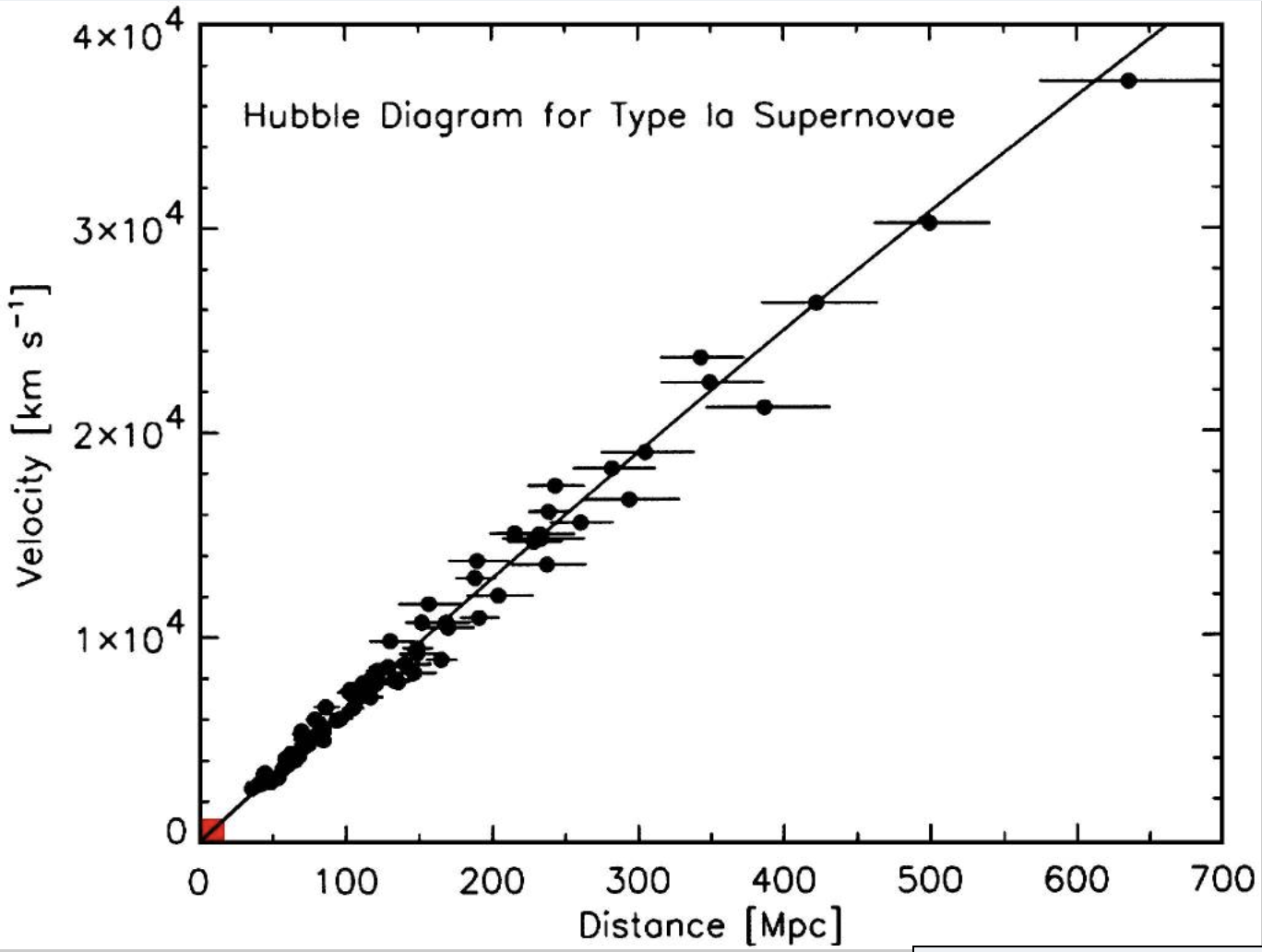
Figure 36.3: The relationship between velocity and distance of stars, using contemporary data in the same format at Edwin Hubble’s 1929 publication.

Each dot in Figure 36.3 is an exploding star called a supernova. The graph shows the relationship between the distance of the star from our galaxy and the outward velocity of that star. The velocities are large, $3 \times 10^4 = 30,000$ km/s is about one-tenth the speed of light. Similarly, the distances are big; 600 Mpc is the same as 2 billion light years or $1.8 \times 10^{22} \text{km}$. The slope of the line in Figure 36.3 is $\frac{3.75 \times 10^4\, \text{km/s}}{1.8 \times 10^{22}\, \text{km}} = 2.1 \times 10^{-18}\, \text{s}^{-1}$. For ease of reading, we will call this slope $\alpha$ and therefore the velocity of a start distance $D$ from Earth is \[v(D) \equiv \alpha D\ .\]

Earlier in the history of the universe each star was a different distance from Earth. We will call this function $D(t)$, distance as a function of time in the universe.

The distance travelled by each star from time $t$ (billions of years ago) to the present is

\[\int_t^\text{now} v(t) dt = D_\text{now} - D(t)\]

which can be re-arranged to give

\[D(t) = D_\text{now} - \int_t^\text{now} v(t) dt .\]

Assuming that $v(t)$ for each star has remained constant at $\alpha D_\text{now}$, the distance travelled by each star since time $t$ depends on its current distance like this:

\[\int_t^\text{now} v(t) dt = \int_t^\text{now} \left[ \alpha D_\text{now}\right]\, dt = \alpha D_\text{now}\left[\text{now} - t\right]\]

Thus, the position of each star at time $t$ is \[D(t) = D_\text{now} - \alpha D_\text{now}\left[\text{now} - t\right] = D(t)\] or,

\[D(t) = D_\text{now}\left({\large\strut} 1-\alpha \left[\text{now} - t\right]\right)\]

According to this model, there was a common time $t_0$ when when all the stars were at the same place: $D(t_0) = 0$. This happened when \[\text{now} - t_0 = \frac{1}{\alpha} = \frac{1}{2.1 \times 10^{-18}\, \text{s}^{-1}} = 4.8 \times 10^{17} \text{s}\ .\] It seems fair to call such a time, when all the stars where at the same place at the same time, as the origin of the universe. If so, $\text{now} - t_0$ corresponds to the age of the universe and our estimate of that age is $4.8\times 10^{17}\text{s}$. Conventionally, this age is reported in years. To get that, we multiply by the flavor of one that turns seconds into years:

\[\frac{60\, \text{seconds}}{1\, \text{minute}} \cdot \frac{60\, \text{minutes}}{1\, \text{hour}} \cdot \frac{24\, \text{hours}}{1\, \text{day}} \cdot \frac{365\, \text{days}}{1\, \text{year}} = 31,500,000 \frac{\text{s}}{\text{year}}\]

The grand (but hypothetical) meeting of the stars therefore occurred $4.8 \times 10^{17} \text{s} / 3.15 \times 10^{7} \text{s/year} = 15,000,000,000$ years ago. Pretty crowded to have all the mass in the universe in one place at the same time. No wonder they call it the Big Bang!

36.5 Exercises

Exercise 36.01

As you know, \[\int_a^c f(x) dx = \int_a^b f(x) dx + \int_b^c f(x) dx\\ \text{and}\\\int_a^c f(x) dx = - \int_c^a f(x) dx\ .\]

Here are some definite integrals for which, without stating anything more about the function, we give you the numerical result.


$\int_{2}^{7} f(x) \,dx = -8$	$\int_{-6}^{-2} g(x) \,dx = 3$
$\int_{2}^{12} f(x) \,dx = -14$	$\int_{0}^{2} g(x) \,dx = 1$
$\int_{2}^{7} h(x) \,dx = 5$	$\int_{0}^{2} h(x) \,dx = 6$

Consider these the facts you have to work with when answering the following questions:

Part A $\int_{2}^{7} 3f(x) \,dx =$?

-8 -42 -24 13

Part B $\int_{7}^{12} f(x) \,dx =$?

6 22 -6 -22

Part C $\int_{2}^{7} f(x) + g(x) \,dx =$?

-3
8
-8
insufficient information to answer question

Part D $\int_{2}^{2} r(x) \,dx =$?

-3
0
-8
insufficient information to answer question at t

Part E $\int_{-6}^{-2} \left[\strut g(x)+3\right] \,dx =$?

6 15 12 3

Part F $\int_{12}^{7} f(x) \,dx =$

-6 22 6 -22

Exercise 36.02

The equation below shows three items, all of which are equivalent even though they look different. You can see this from the equal signs separating the three items.

\[\large \int_{\color{brown}{a}}^{\color{brown}{b}} {\color{blue}{f(x)}}\, dx = {\color{magenta}{F(x)}}\left.{\LARGE\strut}\right|_{\color{brown}{a}}^{\color{brown}{b}} = {\color{magenta}{F}({\color{brown}{b}})} -{\color{magenta}{F}({\color{brown}{a}})}\]

When you reach the point where you can say, “That’s obvious,” and can write down the three items from memory, you will have achieved an important facility with calculus.

Part A Since the three items are equivalent, they are all the same kind of “thing.” What kind of thing are they?

a quantity
a function of $x$
an interval
an integration bound
an anti-derivative
a constant of integration

The equation has been written in color to help you identify elements that are the same in each of the three items.

Part B Which of the colors stands for a bound of integration?

black blue brown magenta

Part C Which of the colors stands for the derivative of a function that appears elsewhere in the equation?

black blue tan magenta

Part D Which of the colors stands for an anti-derivative of a function that appears elsewhere in the equation?

black blue tan magenta

Exercise 36.03

Remember our conventions for notation:

Fixed quantities (perhaps with units)
- Symbols: e.g. $a$, $b$, $c$, $x_0$, $t^{\star}$
- Examples: 3.2, 4.8 meters, 17 feet/sec$^2$
Names of inputs to functions
- Symbols: e.g. $x$, $t$, $y$, $u$, $v$
- Examples: position, time, velocity
Functions of an input
- Symbols: e.g. $f(x)$, $g(t)$, $h(x, t)$
- Examples: position as a function of time, density as a function of position
Functions evaluated at a specific numerical input
- Symbols: e.g. $f(a)$, $g(t_0)$, $h(x^{\star}, t^{\star})$
- Examples: velocity at the finish line, starting position

In particular, take care to distinguish between these two kinds of symbolic items:

$f(x)$, which means $f()$ as a function of $x$
$f(x_0)$, which means the function $f()$ evaluated at the specific input $x_0$, producing a quantity (e.g., 3.5 meters/sec.)

A major source of confusion for students is that $a$ is a constant, even though we are not yet saying specifically which numerical value that constant has. Think of $a$ as meaning “insert constant here.” In terms of derivatives …

$\partial_x f(a) = 0$
$\partial_x f(x)$ is a function
$\partial_u f(x) = 0$, since $u$ and $x$ are different input names.
$\partial_u f(u)$ is a function, the exact same function as in (ii).

With this in mind, turn to our three perspectives on a definite integral \[\large \int_{\color{brown}{a}}^{\color{brown}{b}} {\color{blue}{f(x)}}\, dx = {\color{magenta}{F(x)}}\left.{\LARGE\strut}\right|_{\color{brown}{a}}^{\color{brown}{b}} = {\color{magenta}{F}({\color{brown}{b}})} -{\color{magenta}{F}({\color{brown}{a}})}\]

$\color{brown}{a}$ and $\color{brown}{b}$ are numerical constants
$\color{blue}{f}(x)$ and $\color{magenta}{F}(x)$ are functions of $x$
$\color{magenta}{F}(\color{brown}{a})$ is the function $\color{magenta}{F}()$ evaluated at the specific input $\color{brown}{a}$, producing a quantity. Likewise $\color{magenta}{F}(\color{brown}{b})$.

Part A What kind of a thing is $F(u)$, according to our notation convention? (Hint: First figure out what kind of thing is $u$, according to the notation conventions.)

a fixed quantity a function of $x$ a function of $u$ a definite integral

Part B What kind of a thing is $F(a)$, according to our notation convention?

a quantity a function of $x$ a function of $u$ a definite integral

Part C What kind of a thing is $F(u) - F(a)$, according to our notation convention?

a quantity a function of $x$ a function of $u$ a definite integral

Part D According to our notation convention, what kind of a thing is \[\int_a^u f(x) dx \text{?}\]

a quantity
a function of both $x$ and $u$
a function of $x$
a function of $u$
a definite integral

Part E According to our notation convention, what kind of a thing is \[\int_u^b f(x) dx \text{?}\]

a number
a function of both x and u
a function of $x$
a function of $u$
a definite integral

Part F According to our notation convention, what kind of a thing is \[\int_u^x f(x) dx \text{?}\]

a number
a function of both x and u
a function of $x$
a function of $u$
a definite integral

Now turn to the entities involved in the so-called “First Fundamental Theorem of Calculus.” (“Fundamental theorem” is a highfalutin way of saying something like, “This isn’t obvious at first glance, and so you should be especially careful to memorize it so that you identify it when you see it.” Another way to state it is, “Every function is the derivative of some anti-derivative.” But you knew that already, since “every function has an anti-derivative.”)

Here are the entities involved, which you will recognize as a slight modification of an earlier statement:

\[\partial_u \int_a^u f(x)dx \ \ =\ \ \partial_u \left. F(x) \right|_a^u \ \ = \ \ \partial_u \left(F(u) - F(a)\right) .\]

Let’s look at the right-most expression $\partial_u \left(F(u) + F(a)\right)$ and exploit the the derivative of a sum is the sum of the derivatives. So …

\[\partial_u \left(F(u) + F(a)\right) = \partial_u F(u) - \partial_u F(a) = \partial_u F(u)\]

Part G Which of the following correctly justifies the step \[\partial_u F(u) - \partial_u F(a) = \partial_u F(u)\ \text{?}\]

$F(a)$ is a constant
$F()$ is an anti-derivative.
$F(b)$ does not appear.
$F(u) = \int f(x) dx$

Taking the left-most and right-most expressions in the above equation, we have

\[\partial_u \int_a^u f(x) dx = \partial_u F(u)\]

Part H Is there an algebraic simplification of $\partial_u F(u)$?

No, because it depends on what $F(u)$ is.
Yes, because $\partial_u F(u)$ is simply $f(u)$.
No, because we could just as easily have written $\partial_x F(x)$
Yes, because it is the same thing as $\partial_x F(x)$

The equation \[\partial_u \int_a^u f(x) dx \ \ = \ \ f(u)\] means that “differentiation undoes integration” or, as we’ve been putting it, “differentiation undoes anti-differentiation.”

Exercise 36.04

In the 1660s, John Boyle made use of then-new instrumentation to measure gas pressure. He discovered what’s now called Boyle’s Law, which says that, at constant temperature in a closed system, pressure times volume is a constant:

\[PV = const\]

In the 1720s, Daniel Fahrenheit developed the first reliable thermometer consisting of a column of mercury in a glass straw. He developed a temperature scale which divided the range from freezing to boiling into 180 small units, which he called “degrees,” as was traditional in measuring angles. (In 1742, Anders Celsius created another scale with freezing at 0 and 100 small units—still called “degrees”—between freezing and boiling.

With the availability of reliable thermometers, scientists started to consider the role of temperature in the relationship between pressure and volume. Their many discoveries were eventually synthesized into a “combined gas law” and then into an “ideal gas law” which famously states:

\[PV = nRT .\]

Here, $n$ is “amount” of gas, quantified as the number of moles of the gas in the container, $T$ is temperature, and $R$ is the “ideal gas constant”:

\[R = 8.314 \text{J}/(\text{K}\ \text{mol})\]

The “mol” cancels out the dimension of $n$, the $K$ cancels out the dimension of $T$, leaving us with $PV$ having the dimension of energy (Joules). The temperature $T$ is measured in degrees Kelvin, which is just like Celsius but moving the location of 0 from freezing to … Well … the hypothetical temperature when $PV=0$, which can be estimated by extrapolating measurements of $PV(T)$ (that is, $PV$ as a function of $T$) to the $T$ where $PV = 0$.

Part A It is convenient to have specific units in mind for pressure and volume. Since $P V$ gives energy, let’s arrange $P$ and $V$ to have units such that when multiplied the result is Joules. What is the expression of the dimension Joule in terms of the SI system, that is, time in seconds, length in meters, and mass in kg? Hint: use the above paragraph and knowing that the units for energy are consistent for potential, kinetic, or other types of energy.

$kg m^2 s^{-2}$ $kg m / s$ $kg^2 m^2 s^3$ $m^2 / s^2$

Part B In the SI units system, volume has units of cubic meters: $m^3$. What are the SI units for pressure in terms of kg, m, and s? The units of your answer to this question times the units for pressure should be equivilent to your answer from the previous question.

$kg m^{-1} s^{-2}$ $kg m^1 s^{-2}$ $kg^2 m^1 s^2$ $m s^2 / kg$

For use in calculus, it is helpful to re-write the Ideal Gas Law in functional form. There are several ways to do this. For instance, if we wanted to measure the number of moles of gas in a container, we could use the function $n(P, V, T) = PV/RT$. Here, we will focus on pressure as a function of the other quantities:

\[P(n, V, T) = nRT/V.\]

Now consider a very simple machine consisting of a cylinder, closed on one end and sealed by a movable piston at the other, as in this picture.

Source: R. Castelnuovo - Own work, CC BY-SA 3.0

The machine in the picture is more complicated than the simple machine we want to model. The picture includes two small valves at the top of the cylinder connected each to a pipe.

Our machine has no valves and no pipes. The cylinder is charged with gas when it is manufactured. After that, nothing material goes in or out of the closed cylinder/piston system.

When you push on the cylinder, the volume available for the gas gets smaller and the pressure increases. When you let the cylinder push on you, the volume available gets bigger and the pressure decreases. The amount of gas, $n$, never changes. For simplicity, we will imagine that $n=1$ and that the gas is N$_2$. This means the mass of the gas is 0.028 kg.

And, to simplify even more, let’s insist that the temperature of the cylinder and its gaseous content does not change from room temperature: 293$^\circ$ Kelvin.

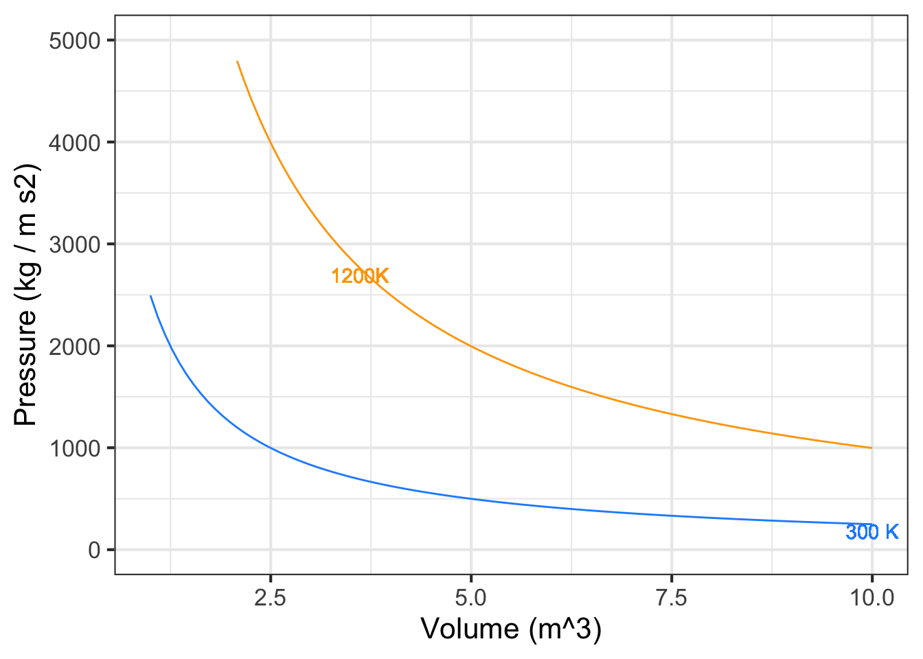
If you start in a high-volume, low-pressure state and push the piston to move to a low-volume, high-pressure state at the same temperature, you will be putting energy into the machine.

The “area” of each little box in the graph, that is, pressure times volume,

Part C How much energy (in Joules) corresponds to one small rectangle of area in the graph?

500 J 625 J 2500 J 25,000 J

Part D By counting rectangles in the graph, estimate how much energy needs to be put into the machine when the volume changes from 7.5 m$^3$ to 2.5 m$^3$ at a temperature of 300 K?

1000 J 3000 J 5000 J 10,000 J

Now that you have compressed the gas in the cylinder, by doing work on it, let’s heat up the machine to 1200K.

Part E What will be the pressure of the gas when the volume of the machine is 2.5 m$^3$ at temperature 1200 K? (The units will be kg m$^{-1} $s^{-2}$)

1000 2000 3000 4000

Part F Starting with the machine at 1200K and a volume of 2.5 m$^3$, how much energy will the machine transfer to you when it expands to 7.5 m$^3$? Estimate this by counting squares in the graph.

about 5000 J about 10,000 J about 50,000 J about 100,000 J

The net work done by the machine in completing the cycle, shifting from compression at low temperature to expansion at high temperature, is the difference between the energy put out by the machine when expanding and the energy put into the machine to compress the gas. Such a machine is called a “heat engine” since it turns a source of high temperature and a source of low temperature into energy.

In a SANDBOX, evaluate the code below. The first line defines a function $P(V, T)$ with default $n=1$ mole of gas. Anti-differentiate $P()$ with respect to $V$ then calculate the energy needed to compress the cylinder at the low temperature, that is \[\int_{7.5}^{2.5} P(V, T=300) dV .\] Call this numerical result compress_energy.

Similarly, calculate the energy done by the machine in the high-temperature expansion \[\int_{2.5}^{7.5} P(V, T=1200) dV .\] Call this numerical result expand_energy.

You may want to make a graph of your $P(V, T)$ function to check that it is right. Also, check that the integrals are right by comparing them to the rough estimate you made earlier by counting squares.

P <- makeFun( n*8.314*T/V ~ V + T, n=1)
antiP <- makeFun(n*8.314*T*log(V) ~ V + T, n=1)

compress_energy <- ... evaluate antiP appropriately
expand_energy   <- ... ditto
compress_energy # prints out the values 
expand_energy

Exercise 36.05

The function windspeed(t) records wind speed at the site of a wind-turbine farm over one day, that is, $0 \leq t \leq 24$ hours. The function speed2power(s) is the production function for the model of wind turbine used at the farm: the input is speed in miles per hour, the output is in kilowatts. (Both these functions were created for this exercise. They are not about a real turbine at a real wind farm, but are somewhat realistic.) Hint: you can nest a function inside of another function. For instance, if I had a function (‘solarpanelpower’) that calculates the amount of power a solar panel generates and another function (‘sunlight’) that tells me the amount of sunlight at time of the day (‘TOD’). I could evaluate this in one step like the following: ‘solarpanelpower(sunlight(TOD))’. This would give me the amount of power from the solar panel based upon the time of the day.

Your task, find the total energy generated over the 24-hour period by the turbine. Reminder: energy $E$ is electric power multiplied by time. Or, more usefully for this problem, the increment energy $dE$ generated at time $t$ is the product of power at time $t$ multiplied by the increment of time $dt$, that is, $dE = p(t) dt$. Consequently, \[E = \int_\text{morning}^\text{night} p(t) dt\] where “morning” should really be 00:00 h and night 24:00 h on the day in question.

We don’t have an algebraic formula for windspeed(t) even though it is a function. You can use antiD() to find the anti-derivative of the electric power function.

The answer you compute should be saved to the name result. The units will be in kWh – kilowatt hours.

# ignore these definitions. They are setting up the 
# functions for you to use
tmp <- rfun(~ t, seed=982)
tmp2 <- rfun(~ t, seed = 2932)
tmp3 <- rfun(~ t, seed = 43)
windspeed <- function(t) {
  abs(tmp((t - 5)*3) + tmp2((t - 10)*2) + tmp3((t - 15)*4))
}
speed2power <- function(s) {
  pmin(ifelse(s < 5, 0, (s-2)^3), 5000)
}

#Your work starts here

slice_plot(windspeed(t) ~ t, bounds(t=c(0, 24)))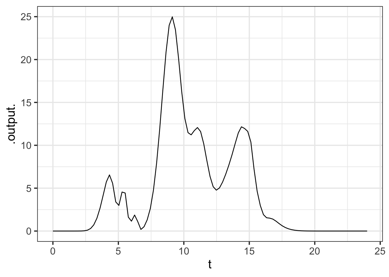


# # Uncomment the next lines as you figure out how to fill in the "...blanks..."
# antid_of_power <- antiD( ....power_function_here(t)... ~ t)
# result <- antid_of_power(...night...) - antid_of_power(...morning...) 
# result # this prints out the result

Part A Wind turbines of this type have a maximum power rating of 5000 kilowatts. Was this rating exceeded at any point during the day?

The maximum instantaneous power was about 3500 kilowatts
The maximum instantaneous power was about 1100 kilowatts
That threshold was reached about 9 AM
That threshold was exceeded about 8 AM
The maximum instantaneous power cannot be determined from the information given.

Part B At the maximum power rating of 5000 kilowatts, what’s the theoretical maximum amount of energy produced by the turbine over a 24-hour day?

5000 * 24 kilowatt-hours
5000 / 24 kilowatt-hours
5000 kilowatts
Can’t be determined from the information given.

Part C About what fraction of the theoretical maximum energy did the wind turbine generate over the 24-hour period?

About 2.5%
About 10%
About 25%
About 50%
Can’t be determined from the information given.

Part D A peak time for residential energy consumption is from 7 am to 9 am. The price at which you can sell electrical energy to the grid operator is $0.09 per kilowatt-hour. At that price, how much would the energy produced from 7-9 am be worth?

About 20 cents. About $150 About $350 About $650

Part E What’s the average wind speed over the 24-hour period?

About 5 mph About 7 mph About 9 mph

Part F Wind speed fluctuates a lot, but imagine that the wind blew steadily at the average wind speed from the previous problem. How much energy would be generated over the 24-hour period?

0 kilowatt hours
500 kilowatt hours
1000 kilowatt hours
10,000 kilowatt hours

Exercise 36.06

The (so-called) “First Fundamental Theorem of Calculus” says:

\[\partial_t \int_a^t f(x) dx \ = \ f(t)\]

Part A Consider this new quantity: \[\partial_t \int_t^a f(x) dx\] Which of the following is a valid simplification of the quantity?

$f(t)$ $f(-t)$ $-f(t)$ none of the above

Exercise 36.07

Your house has solar panels on the roof. In sunshine, these generate power. You use some of that power immediately for cooking, lighting, and such. Any power generated above your needs gets stored in a battery. Any power used above the solar generation gets supplied by the battery.

Over the course of a day, your use of power fluctuates (you use the toaster, open the refrigerator, etc). Similarly, the solar generation fluctuates as clouds pass by and the sun rises and sets in the sky. The amount of energy stored in the battery fluctuates over the day as you consume energy in your home and produce it with the solar panels.

The unit used for electrical power is a “kilowatt” (kW). An old-fashioned incandescent light bulb consumes about 0.1 kW while lighted, a modern LED bulb generates about the same amount of light using only 0.01 kW. A refrigerator uses about 0.1 kW while a hair-dryer uses about 1 kW when it is running.

Batteries store energy. The usual unit for energy is “kilowatt-hour” (kWh). A refrigerator will, over a 24-hour day, use 0.1 * 24 = 2.4 kWh. Power multiplied by time duration gives energy. If the power were constant, the energy could be calculated by a simple multiplication of the power over the duration. Since power fluctuates, we cannot do the calculation with ordinary multiplication. Instead, we have to integrate power over time.

For this activity, use the “Solar-panels” App.

Add picture/link to app.

Part A Why is it called “net production” instead of just “production?”

Because your house is connected to the utility electrical network in case you need extra power.
Because the system designer is something of a poet and wants you to think of the solar cells as a kind of fishing net harvesting photons.
Because the government will send you surplus hair nets to thank you for reducing CO2 production.
Because it is not simply production from the solar panels but production minus consumption (the solar panels require energy to run). If you ignored consumption, you would call it “gross energy produced.”

Part B The bottom graph shows energy accumulated in the battery since midnight. What does it mean that the energy accumulated is negative?

The battery level is lower throughout the day than it was at midnight.
The battery is discharging over the entire day.
The sign is not important.

Part C During the interval from 05:00 to 20:00, how much did the energy stored by the battery change? Highlight that interval in the beeps graph.

-2.5 kWh 1.9 kW 15 hours 1.5 kWh

Part D Suppose the battery was holding 20 kWh at 00:00. How much energy was it holding at 15:00?

-2 kWh 18 kWh 20 kWh 24 kWh

Part E When you choose a time interval in the beep graph, how come the energy stored (in kWh) is displayed as an area in the top graph? Keep in mind that the vertical scale of the top graph is kW, not kWh.

It is pretty.
To highlight visually the interval that was selected.
To convert kW to kWh, we are effectively multiplying the power (kW) by the time duration. Power is on the vertical axis, time duration is on the horizontal axis. Multiplying the two corresponds to the area under the graph.

Part F How come two different colors are used to display the “area” under the net power curve?

The second derivative of the anti-derivative of $f(t)$ is equal to $f(t)$.
No reason related to calculus per se. We like to make graphs pretty.
Because it is not simply “area.” it is the product of net power and time duration, and sometimes this quantity is negative. The color indicates whether the quantity is positive or negative at any instant.

Exercise 36.08

Suppose the continuous function $f(x)$ is positive on $x \in [0, 4]$ and negative on $x \in [4, 8]$. Let \[F(x) \equiv \int_0^x f(u) du.\] In addition, suppose $\int_0^8 f(x)dx < 0$.

Mark each statement as True or False.

Part A $F(x)$ has to be positive on [0,4] and negative on [4, 8].

True False

Part B $F(x)$ must cross the x-axis at least once in the interval [0, 8].

True False

Part C $F(0) < F(8)$.

True False

Part D $F(x)$ is concave up on [0, 4] and concave down on [4, 8].

True False

Part E $F(x)$ has a local maximum at x = 4.

True False

Part F $F(x)$ has a point of inflection at x=4.

True False

Exercise 36.09

Part A Which of the following is NOT equivalent to \[\int_1^4\frac{1}{x}dx\ ?\]

$\ln|x| {\Large|_{\tiny 1}^{\tiny 4}}$
$1.386294$
$\ln|4|-\ln|1|$
$\frac {x^0}{0} {\Large|_{\tiny 1}^{\tiny 4}}$

Exercise 36.10

Part A Find the antiderivative \[\int \frac{x^2+x+1}{x}\ dx\ .\]

$\frac{1}{2} x^2+x+\ln(|x|)+C$
$\frac{\frac{1}{3} x^3+\frac{1}{2} x^2 +x}{\frac{1}{2}x^2}+C$
$x\cdot(\frac{1}{3} x^3+\frac{1}{2} x^2 +x)-(x^2+x+1)\cdot (\frac{1}{2} x^2)+C$

Part B Find the antiderivative \[\int \left(\frac{3}{t} - \frac{3}{t^2} \right)dt\ .\]

$3\ln(t)+\frac{2}{t} +C$
$3\ln|t|+\frac{2}{t} +C$
$\frac{-3}{2t^2}+\frac 2 {3t^3} +C$
$\frac{-3}{\frac{1}{2} t^2}+\frac {2}{\frac{1}{3} {t^3}} +C$

Part C Find the value of \[\int_2^4(2x+3)dx\ .\]

$-18$ $4$ $12$ $18$

Part D What is the approximate value of \[\int_2^4 dnorm(x)dx\ ?\] (Hint: You will need an R session to do the numerical calculation.

$0.02271846$ $-0.02271846$ $-0.05385714$ $1.977218$

Problem with Accumulation Exercises/buck-forgive-canoe.Rmd

Problem with Accumulation Exercises/horse-drive-futon.Rmd

Momentum is velocity times mass. Newton’s Second Law of Motion stipulates that force equals the rate of change of momentum.↩︎

Context	Quantity	Rate of increase in quantity
Money	Cash on hand \({\mathbf S}(t)\)	Cash flow \(s(t)\)
Fuel	Amount in fuel tank \({\mathbf F}(t)\)	Fuel consumption rate, e.g. kg/hour \(f(t)\)
Motion	Momentum \({\mathbf M}(t)\)	Force \(m(t)\)
notation	\({\mathbf H}(t)\)	\(\partial_t {\mathbf H}(t)\)
notation	\(G(t) = \int g(t) dt\)	\(g(t)\)


\(\int_{2}^{7} f(x) \,dx = -8\)	\(\int_{-6}^{-2} g(x) \,dx = 3\)
\(\int_{2}^{12} f(x) \,dx = -14\)	\(\int_{0}^{2} g(x) \,dx = 1\)
\(\int_{2}^{7} h(x) \,dx = 5\)	\(\int_{0}^{2} h(x) \,dx = 6\)