Count and density histograms in ggformula.
Usage
gf_histogram(
  object = NULL,
  gformula = NULL,
  data = NULL,
  ...,
  bins,
  binwidth,
  alpha = 0.5,
  color,
  fill,
  group,
  linetype,
  linewidth,
  xlab,
  ylab,
  title,
  subtitle,
  caption,
  geom = "bar",
  stat = "bin",
  position = "stack",
  show.legend = NA,
  show.help = NULL,
  inherit = TRUE,
  environment = parent.frame()
)

gf_dhistogram(
  object = NULL,
  gformula = NULL,
  data = NULL,
  ...,
  bins,
  binwidth,
  alpha = 0.5,
  color,
  fill,
  group,
  linetype,
  linewidth,
  xlab,
  ylab,
  title,
  subtitle,
  caption,
  geom = "bar",
  stat = "bin",
  position = "stack",
  show.legend = NA,
  show.help = NULL,
  inherit = TRUE,
  environment = parent.frame()
)
Arguments
- object
When chaining, this holds an object produced in the earlier portions of the chain. Most users can safely ignore this argument. See details and examples.
- gformula
A formula with shape
~ x(ory ~ x, but this shape is not generally needed).- data
The data to be displayed in this layer. There are three options:
If
NULL, the default, the data is inherited from the plot data as specified in the call toggplot().A
data.frame, or other object, will override the plot data. All objects will be fortified to produce a data frame. Seefortify()for which variables will be created.A
functionwill be called with a single argument, the plot data. The return value must be adata.frame, and will be used as the layer data. Afunctioncan be created from aformula(e.g.~ head(.x, 10)).- ...
Additional arguments. Typically these are (a) ggplot2 aesthetics to be set with
attribute = value, (b) ggplot2 aesthetics to be mapped withattribute = ~ expression, or (c) attributes of the layer as a whole, which are set withattribute = value.- bins
Number of bins. Overridden by
binwidth. Defaults to 30.- binwidth
The width of the bins. Can be specified as a numeric value or as a function that takes x after scale transformation as input and returns a single numeric value. When specifying a function along with a grouping structure, the function will be called once per group. The default is to use the number of bins in
bins, covering the range of the data. You should always override this value, exploring multiple widths to find the best to illustrate the stories in your data.The bin width of a date variable is the number of days in each time; the bin width of a time variable is the number of seconds.
- alpha
Opacity (0 = invisible, 1 = opaque).
- color
A color or a formula used for mapping color.
- fill
A color for filling, or a formula used for mapping fill.
- group
Used for grouping.
- linetype
A linetype (numeric or "dashed", "dotted", etc.) or a formula used for mapping linetype.
- linewidth
A numerical line width or a formula used for mapping linewidth.
- xlab
Label for x-axis. See also
gf_labs().- ylab
Label for y-axis. See also
gf_labs().- title, subtitle, caption
Title, sub-title, and caption for the plot. See also
gf_labs().- geom, stat
Use to override the default connection between
geom_histogram()/geom_freqpoly()andstat_bin(). For more information at overriding these connections, see how the stat and geom arguments work.- position
A position adjustment to use on the data for this layer. This can be used in various ways, including to prevent overplotting and improving the display. The
positionargument accepts the following:The result of calling a position function, such as
position_jitter(). This method allows for passing extra arguments to the position.A string naming the position adjustment. To give the position as a string, strip the function name of the
position_prefix. For example, to useposition_jitter(), give the position as"jitter".For more information and other ways to specify the position, see the layer position documentation.
- show.legend
logical. Should this layer be included in the legends?
NA, the default, includes if any aesthetics are mapped.FALSEnever includes, andTRUEalways includes. It can also be a named logical vector to finely select the aesthetics to display. To include legend keys for all levels, even when no data exists, useTRUE. IfNA, all levels are shown in legend, but unobserved levels are omitted.- show.help
If
TRUE, display some minimal help.- inherit
A logical indicating whether default attributes are inherited.
- environment
An environment in which to look for variables not found in
data.
Specifying plot attributes
Positional attributes (a.k.a, aesthetics) are specified using the formula in gformula.
Setting and mapping of additional attributes can be done through the
use of additional arguments.
Attributes can be set can be set using arguments of the form attribute = value or
mapped using arguments of the form attribute = ~ expression.
In formulas of the form A | B, B will be used to form facets using
ggplot2::facet_wrap() or ggplot2::facet_grid().
This provides an alternative to
gf_facet_wrap() and
gf_facet_grid() that is terser and may feel more familiar to users
of lattice.
Evaluation
Evaluation of the ggplot2 code occurs in the environment of gformula.
This will typically do the right thing when formulas are created on the fly, but might not
be the right thing if formulas created in one environment are used to create plots
in another.
Examples
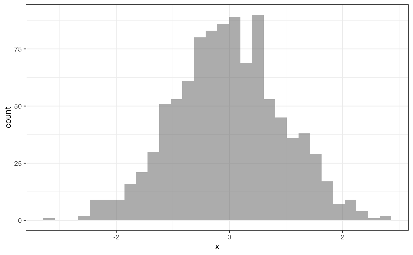
x <- rnorm(1000)
gf_histogram(~x, bins = 30)
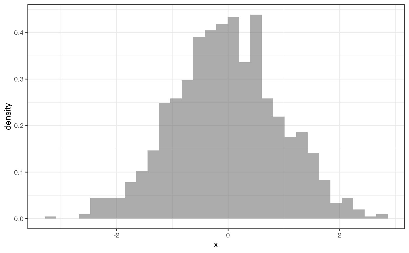
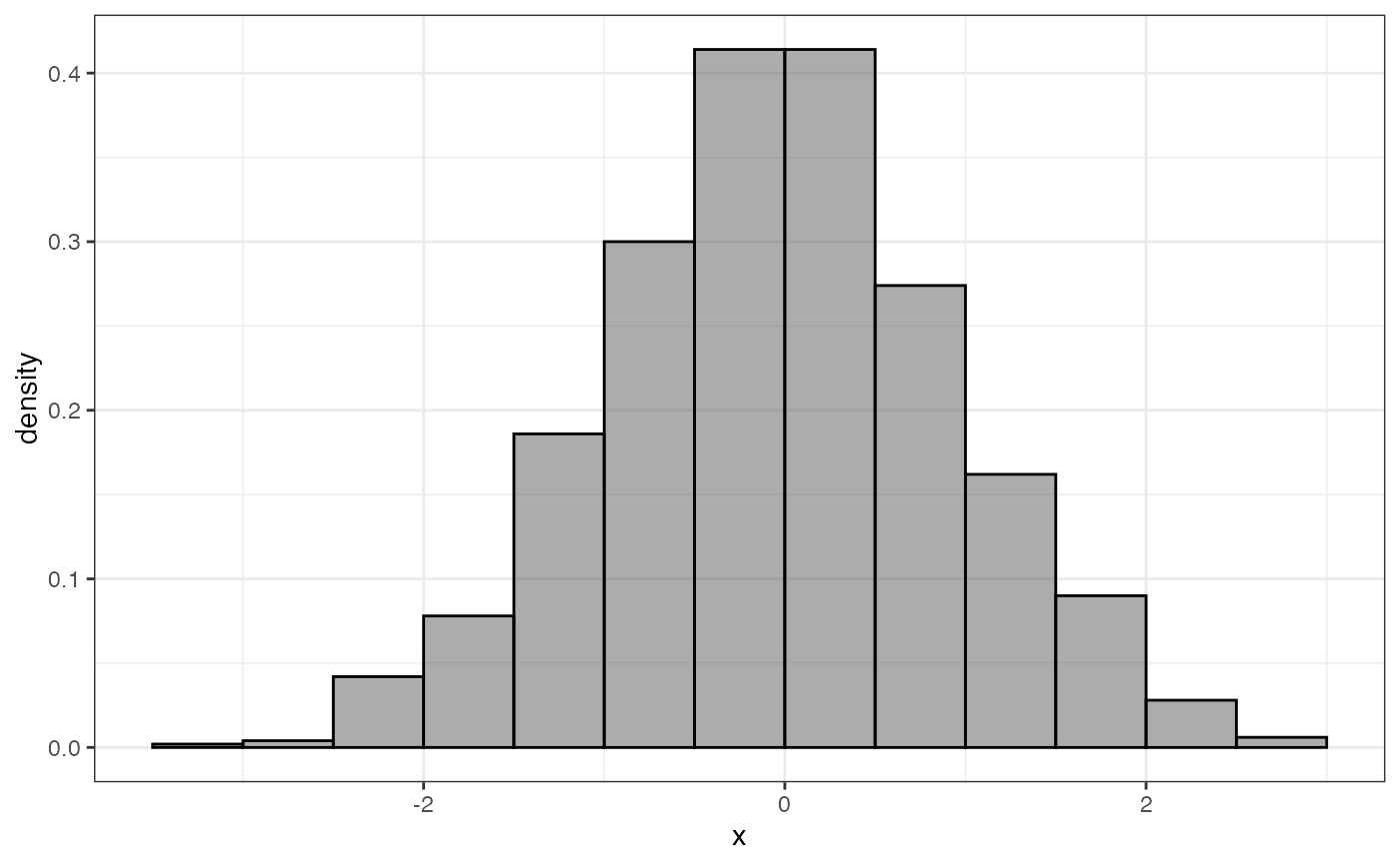
 gf_dhistogram(~x, bins = 30)
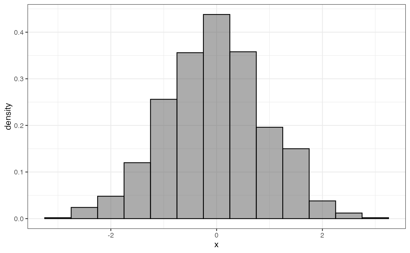
 gf_dhistogram(~x, binwidth = 0.5, center = 0, color = "black", bins = 30)
 gf_dhistogram(~x, binwidth = 0.5, boundary = 0, color = "black", bins = 30)
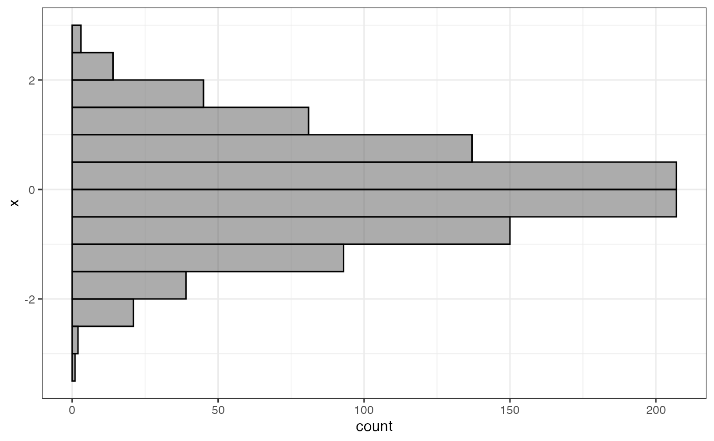
 gf_dhistogram(x ~ ., binwidth = 0.5, boundary = 0, color = "black", bins = 30)
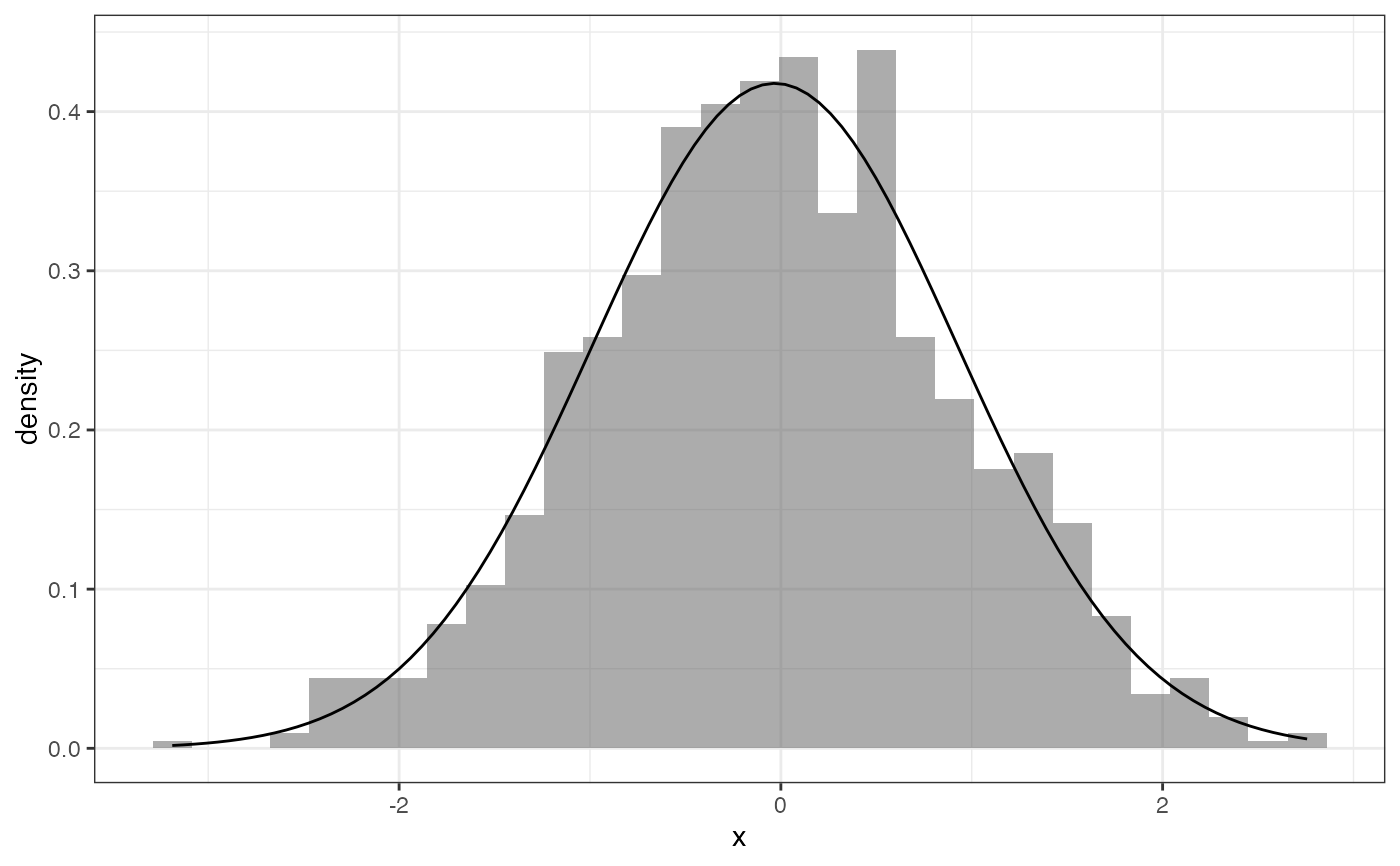
 gf_dhistogram(~x, bins = 30) |>
gf_fitdistr(dist = "dnorm") # see help for gf_fitdistr() for more info.
gf_dhistogram(~x, bins = 30) |>
gf_fitdistr(dist = "dnorm") # see help for gf_fitdistr() for more info.
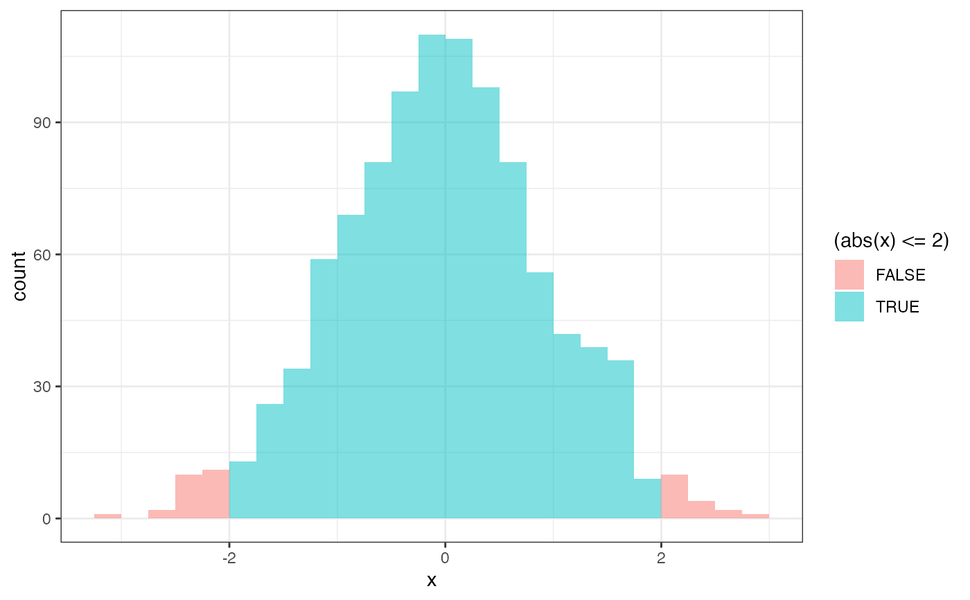
 gf_histogram(~x, fill = ~ (abs(x) <= 2), boundary = 2, binwidth = 0.25)
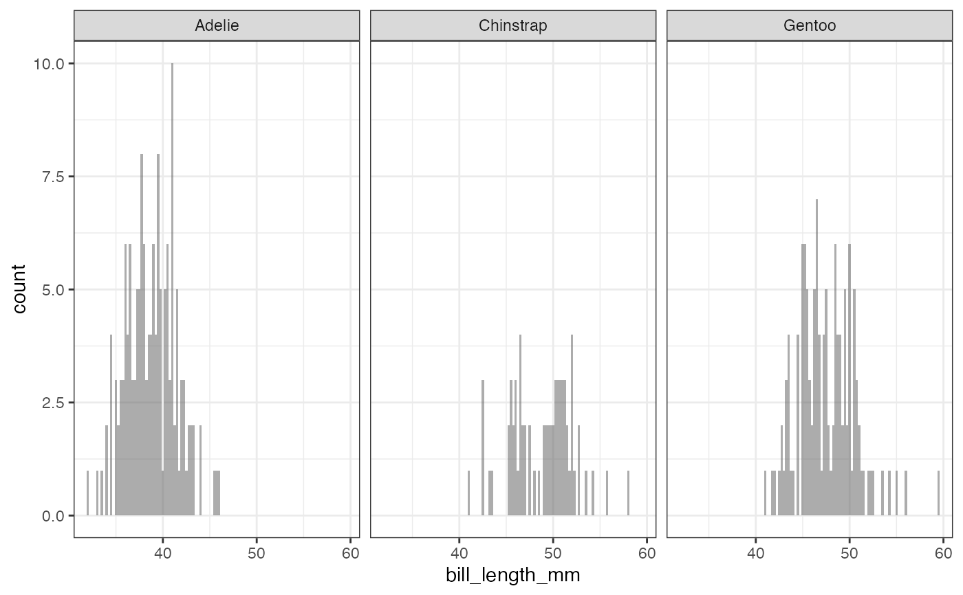
 data(penguins, package = "palmerpenguins")
gf_histogram(~ bill_length_mm | species, data = penguins, binwidth = 0.25)
#> Warning: Removed 2 rows containing non-finite outside the scale range (`stat_bin()`).
data(penguins, package = "palmerpenguins")
gf_histogram(~ bill_length_mm | species, data = penguins, binwidth = 0.25)
#> Warning: Removed 2 rows containing non-finite outside the scale range (`stat_bin()`).
 gf_histogram(~age,
data = mosaicData::HELPrct, binwidth = 5,
fill = "skyblue", color = "black"
)
gf_histogram(~age,
data = mosaicData::HELPrct, binwidth = 5,
fill = "skyblue", color = "black"
)
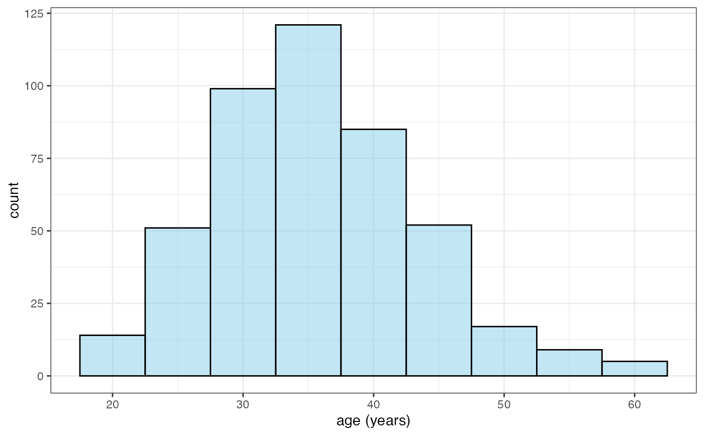 # bins can be adjusted left/right using center or boundary
gf_histogram(~age,
data = mosaicData::HELPrct,
binwidth = 5, fill = "skyblue", color = "black", center = 42.5
)
# bins can be adjusted left/right using center or boundary
gf_histogram(~age,
data = mosaicData::HELPrct,
binwidth = 5, fill = "skyblue", color = "black", center = 42.5
)
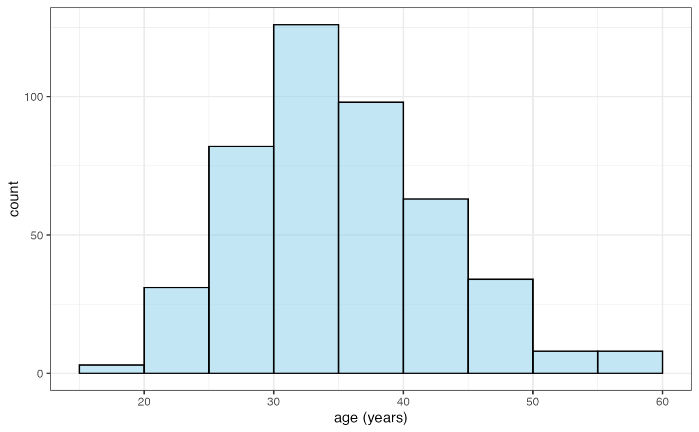 gf_histogram(~age,
data = mosaicData::HELPrct,
binwidth = 5, fill = "skyblue", color = "black", boundary = 40
)
gf_histogram(~age,
data = mosaicData::HELPrct,
binwidth = 5, fill = "skyblue", color = "black", boundary = 40
)
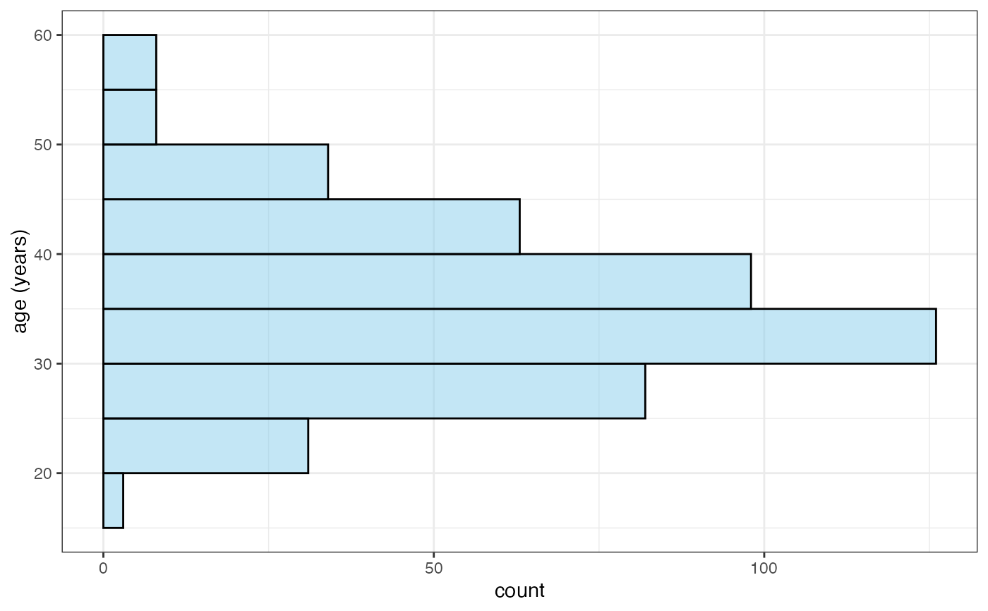
 gf_histogram(age ~ .,
data = mosaicData::HELPrct,
binwidth = 5, fill = "skyblue", color = "black", boundary = 40
)
gf_histogram(age ~ .,
data = mosaicData::HELPrct,
binwidth = 5, fill = "skyblue", color = "black", boundary = 40
)