Formula interface to geom_linerange() and geom_pointrange()
Source:R/gf_functions.R
gf_linerange.RdVarious ways of representing a vertical interval defined by x,
ymin and ymax. Each case draws a single graphical object.
Usage
gf_linerange(
  object = NULL,
  gformula = NULL,
  data = NULL,
  ...,
  alpha,
  color,
  group,
  linetype,
  linewidth,
  xlab,
  ylab,
  title,
  subtitle,
  caption,
  geom = "linerange",
  stat = "identity",
  position = "identity",
  show.legend = NA,
  show.help = NULL,
  inherit = TRUE,
  environment = parent.frame()
)

gf_pointrange(
  object = NULL,
  gformula = NULL,
  data = NULL,
  ...,
  alpha,
  color,
  group,
  linetype,
  linewidth,
  size,
  xlab,
  ylab,
  title,
  subtitle,
  caption,
  geom = "pointrange",
  stat = "identity",
  position = "identity",
  show.legend = NA,
  show.help = NULL,
  inherit = TRUE,
  environment = parent.frame()
)

gf_summary(
  object = NULL,
  gformula = NULL,
  data = NULL,
  ...,
  alpha,
  color,
  group,
  linetype,
  linewidth = 1,
  size,
  fun.y = NULL,
  fun.ymax = NULL,
  fun.ymin = NULL,
  fun.args = list(),
  xlab,
  ylab,
  title,
  subtitle,
  caption,
  geom = "pointrange",
  stat = "summary",
  position = "identity",
  show.legend = NA,
  show.help = NULL,
  inherit = TRUE,
  environment = parent.frame()
)
Arguments
- object
When chaining, this holds an object produced in the earlier portions of the chain. Most users can safely ignore this argument. See details and examples.
- gformula
A formula with shape
ymin + ymax ~ x. Faceting can be achieved by including|in the formula.- data
The data to be displayed in this layer. There are three options:
If
NULL, the default, the data is inherited from the plot data as specified in the call toggplot().A
data.frame, or other object, will override the plot data. All objects will be fortified to produce a data frame. Seefortify()for which variables will be created.A
functionwill be called with a single argument, the plot data. The return value must be adata.frame, and will be used as the layer data. Afunctioncan be created from aformula(e.g.~ head(.x, 10)).- ...
Additional arguments. Typically these are (a) ggplot2 aesthetics to be set with
attribute = value, (b) ggplot2 aesthetics to be mapped withattribute = ~ expression, or (c) attributes of the layer as a whole, which are set withattribute = value.- alpha
Opacity (0 = invisible, 1 = opaque).
- color
Set or map color.
- group
Use to set or map group.
- linetype, linewidth
Set or map style of the line.
- xlab
Label for x-axis. See also
gf_labs().- ylab
Label for y-axis. See also
gf_labs().- title, subtitle, caption
Title, sub-title, and caption for the plot. See also
gf_labs().- geom
The geometric object to use to display the data for this layer. When using a
stat_*()function to construct a layer, thegeomargument can be used to override the default coupling between stats and geoms. Thegeomargument accepts the following:A
Geomggproto subclass, for exampleGeomPoint.A string naming the geom. To give the geom as a string, strip the function name of the
geom_prefix. For example, to usegeom_point(), give the geom as"point".For more information and other ways to specify the geom, see the layer geom documentation.
- stat
The statistical transformation to use on the data for this layer. When using a
geom_*()function to construct a layer, thestatargument can be used to override the default coupling between geoms and stats. Thestatargument accepts the following:A
Statggproto subclass, for exampleStatCount.A string naming the stat. To give the stat as a string, strip the function name of the
stat_prefix. For example, to usestat_count(), give the stat as"count".For more information and other ways to specify the stat, see the layer stat documentation.
- position
A position adjustment to use on the data for this layer. This can be used in various ways, including to prevent overplotting and improving the display. The
positionargument accepts the following:The result of calling a position function, such as
position_jitter(). This method allows for passing extra arguments to the position.A string naming the position adjustment. To give the position as a string, strip the function name of the
position_prefix. For example, to useposition_jitter(), give the position as"jitter".For more information and other ways to specify the position, see the layer position documentation.
- show.legend
logical. Should this layer be included in the legends?
NA, the default, includes if any aesthetics are mapped.FALSEnever includes, andTRUEalways includes. It can also be a named logical vector to finely select the aesthetics to display. To include legend keys for all levels, even when no data exists, useTRUE. IfNA, all levels are shown in legend, but unobserved levels are omitted.- show.help
If
TRUE, display some minimal help.- inherit
A logical indicating whether default attributes are inherited.
- environment
An environment in which to look for variables not found in
data.- size
size aesthetic for points (
gf_pointrange()).- fun.ymin, fun.y, fun.ymax
![[Deprecated]](figures/lifecycle-deprecated.svg) Use the
versions specified above instead.
Use the
versions specified above instead.- fun.args
Optional additional arguments passed on to the functions.
Examples
gf_linerange()
#> gf_linerange() uses
#> * a formula with shape ymin + ymax ~ x or y ~ xmin + xmax.
#> * geom: linerange
#> * key attributes: alpha, color, group, linetype, linewidth
#>
#> For more information, try ?gf_linerange
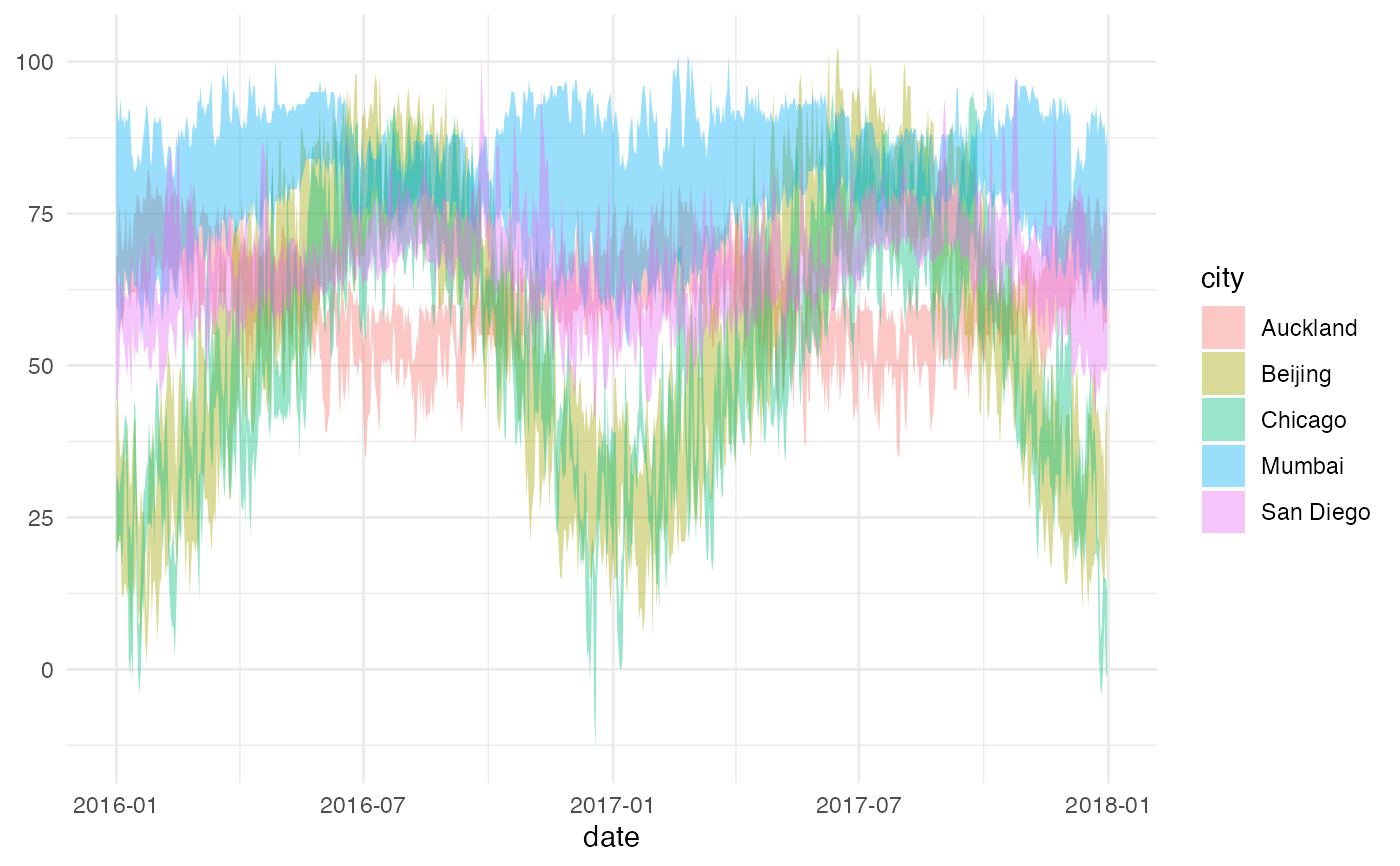
gf_ribbon(low_temp + high_temp ~ date,
data = mosaicData::Weather,
fill = ~city, alpha = 0.4
) |>
gf_theme(theme = theme_minimal())
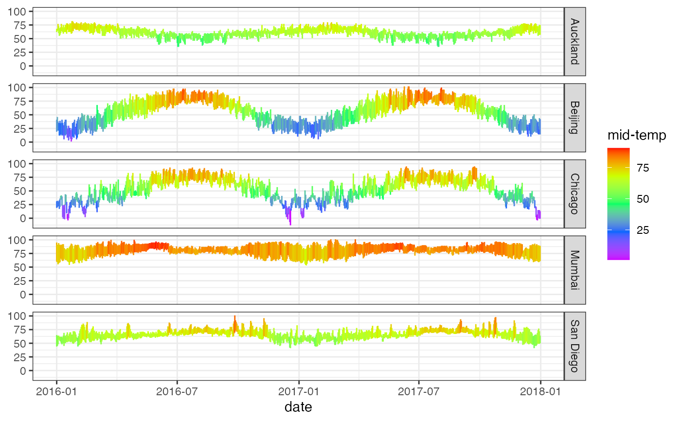
 gf_linerange(
low_temp + high_temp ~ date | city ~ .,
data = mosaicData::Weather,
color = ~ ((low_temp + high_temp) / 2)
) |>
gf_refine(scale_colour_gradientn(colors = rev(rainbow(5)))) |>
gf_labs(color = "mid-temp")
gf_linerange(
low_temp + high_temp ~ date | city ~ .,
data = mosaicData::Weather,
color = ~ ((low_temp + high_temp) / 2)
) |>
gf_refine(scale_colour_gradientn(colors = rev(rainbow(5)))) |>
gf_labs(color = "mid-temp")
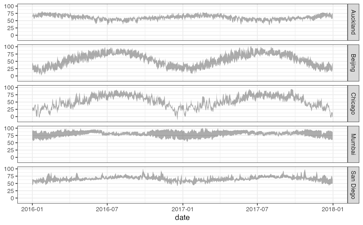
 gf_ribbon(low_temp + high_temp ~ date | city ~ ., data = mosaicData::Weather)
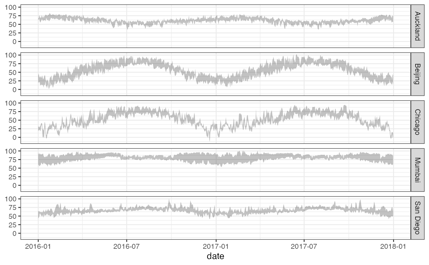 # Chaining in the data
mosaicData::Weather |>
gf_ribbon(low_temp + high_temp ~ date, alpha = 0.4) |>
gf_facet_grid(city ~ .)
# Chaining in the data
mosaicData::Weather |>
gf_ribbon(low_temp + high_temp ~ date, alpha = 0.4) |>
gf_facet_grid(city ~ .)
 if (require(mosaicData) && require(dplyr)) {
HELP2 <- HELPrct |>
group_by(substance, sex) |>
summarise(
mean.age = mean(age),
median.age = median(age),
max.age = max(age),
min.age = min(age),
sd.age = sd(age),
lo = mean.age - sd.age,
hi = mean.age + sd.age
)
gf_jitter(age ~ substance, data = HELPrct,
alpha = 0.5, width = 0.2, height = 0, color = "skyblue") |>
gf_pointrange(mean.age + lo + hi ~ substance, data = HELP2) |>
gf_facet_grid(~sex)
gf_jitter(age ~ substance, data = HELPrct,
alpha = 0.5, width = 0.2, height = 0, color = "skyblue") |>
gf_errorbar(lo + hi ~ substance, data = HELP2, inherit = FALSE) |>
gf_facet_grid(~sex)
# width is defined differently for gf_boxplot() and gf_jitter()
# * for gf_boxplot() it is the full width of the box.
# * for gf_jitter() it is half that -- the maximum amount added or subtracted.
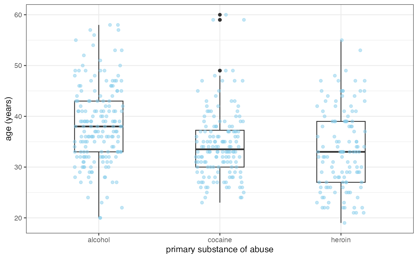
gf_boxplot(age ~ substance, data = HELPrct, width = 0.4) |>
gf_jitter(width = 0.4, height = 0, color = "skyblue", alpha = 0.5)
gf_boxplot(age ~ substance, data = HELPrct, width = 0.4) |>
gf_jitter(width = 0.2, height = 0, color = "skyblue", alpha = 0.5)
}
#> `summarise()` has grouped output by 'substance'. You can override using the
#> `.groups` argument.
if (require(mosaicData) && require(dplyr)) {
HELP2 <- HELPrct |>
group_by(substance, sex) |>
summarise(
mean.age = mean(age),
median.age = median(age),
max.age = max(age),
min.age = min(age),
sd.age = sd(age),
lo = mean.age - sd.age,
hi = mean.age + sd.age
)
gf_jitter(age ~ substance, data = HELPrct,
alpha = 0.5, width = 0.2, height = 0, color = "skyblue") |>
gf_pointrange(mean.age + lo + hi ~ substance, data = HELP2) |>
gf_facet_grid(~sex)
gf_jitter(age ~ substance, data = HELPrct,
alpha = 0.5, width = 0.2, height = 0, color = "skyblue") |>
gf_errorbar(lo + hi ~ substance, data = HELP2, inherit = FALSE) |>
gf_facet_grid(~sex)
# width is defined differently for gf_boxplot() and gf_jitter()
# * for gf_boxplot() it is the full width of the box.
# * for gf_jitter() it is half that -- the maximum amount added or subtracted.
gf_boxplot(age ~ substance, data = HELPrct, width = 0.4) |>
gf_jitter(width = 0.4, height = 0, color = "skyblue", alpha = 0.5)
gf_boxplot(age ~ substance, data = HELPrct, width = 0.4) |>
gf_jitter(width = 0.2, height = 0, color = "skyblue", alpha = 0.5)
}
#> `summarise()` has grouped output by 'substance'. You can override using the
#> `.groups` argument.
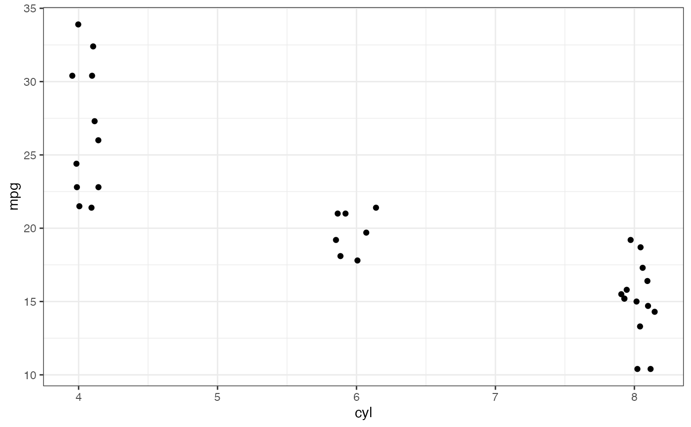
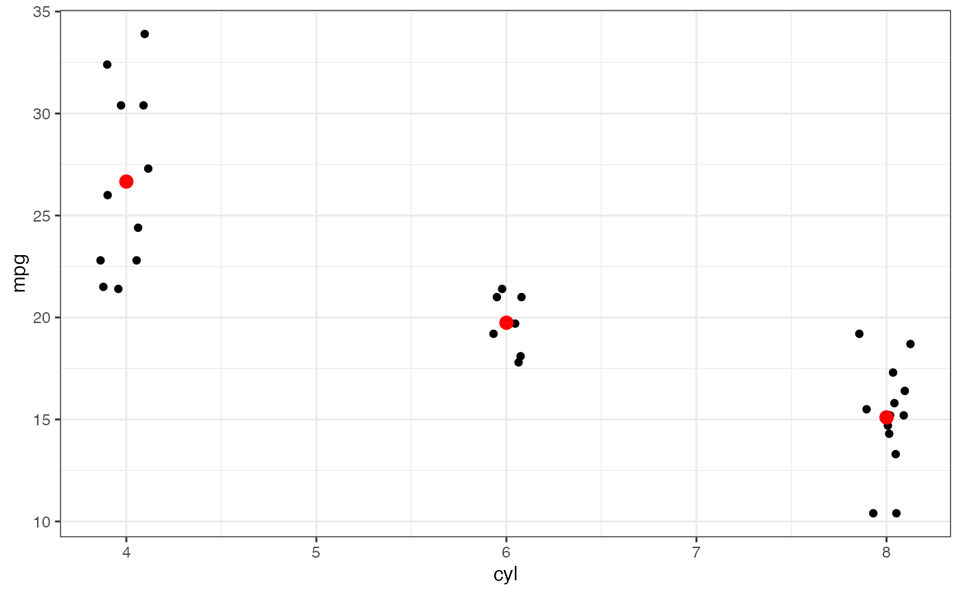
 p <- gf_jitter(mpg ~ cyl, data = mtcars, height = 0, width = 0.15); p
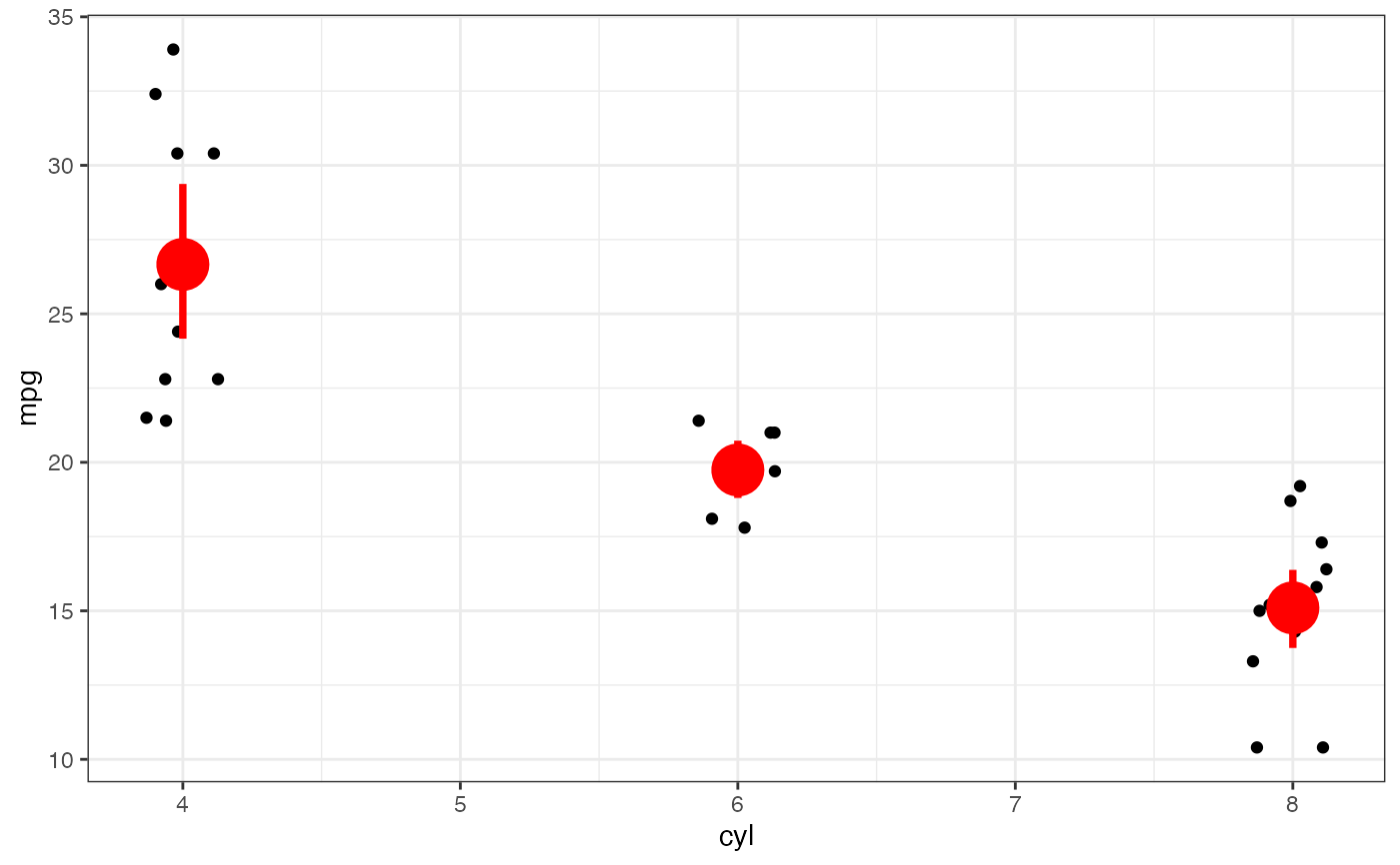
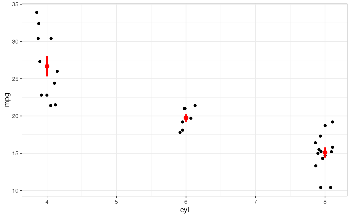
 p |> gf_summary(fun.data = "mean_cl_boot", color = "red", size = 2, linewidth = 1.3)
 # You can supply individual functions to summarise the value at
# each x:
p |> gf_summary(fun.y = "median", color = "red", size = 3, geom = "point")
#> No summary function supplied, defaulting to `mean_se()`
# You can supply individual functions to summarise the value at
# each x:
p |> gf_summary(fun.y = "median", color = "red", size = 3, geom = "point")
#> No summary function supplied, defaulting to `mean_se()`
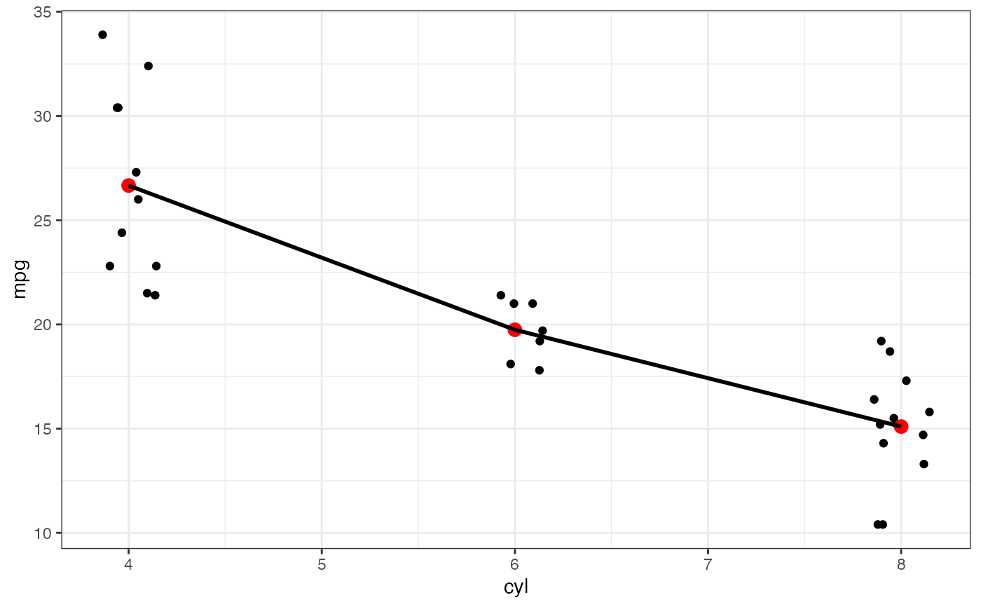
 p |>
gf_summary(fun.y = "mean", color = "red", size = 3, geom = "point") |>
gf_summary(fun.y = mean, geom = "line")
#> No summary function supplied, defaulting to `mean_se()`
#> No summary function supplied, defaulting to `mean_se()`
p |>
gf_summary(fun.y = "mean", color = "red", size = 3, geom = "point") |>
gf_summary(fun.y = mean, geom = "line")
#> No summary function supplied, defaulting to `mean_se()`
#> No summary function supplied, defaulting to `mean_se()`
 p |>
gf_summary(fun.y = mean, fun.ymin = min, fun.ymax = max, color = "red")
#> No summary function supplied, defaulting to `mean_se()`
p |>
gf_summary(fun.y = mean, fun.ymin = min, fun.ymax = max, color = "red")
#> No summary function supplied, defaulting to `mean_se()`
 if (FALSE) { # \dontrun{
p |>
gf_summary(fun.ymin = min, fun.ymax = max, color = "red", geom = "linerange")
} # }
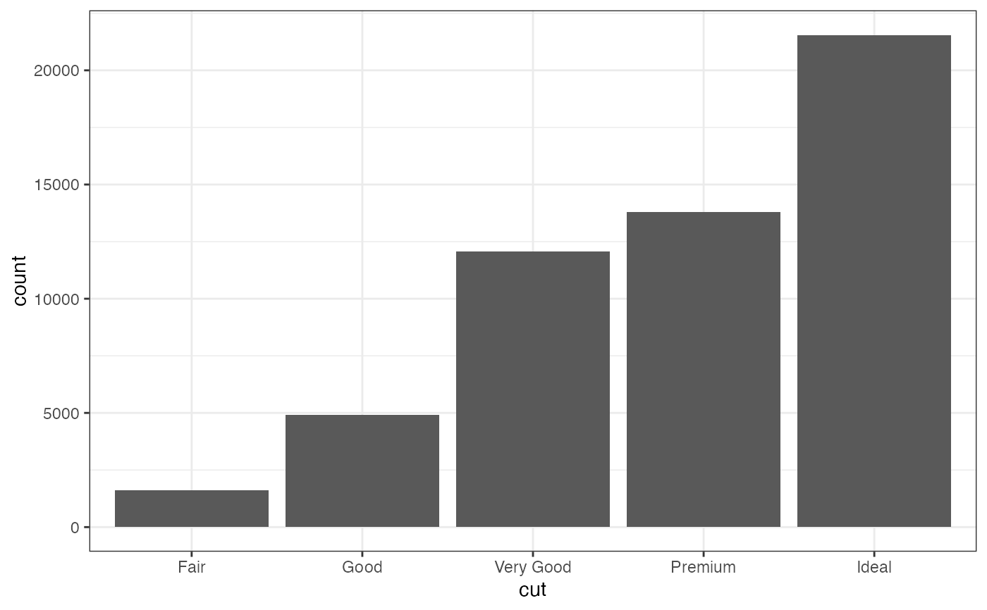
gf_bar(~ cut, data = diamonds)
if (FALSE) { # \dontrun{
p |>
gf_summary(fun.ymin = min, fun.ymax = max, color = "red", geom = "linerange")
} # }
gf_bar(~ cut, data = diamonds)
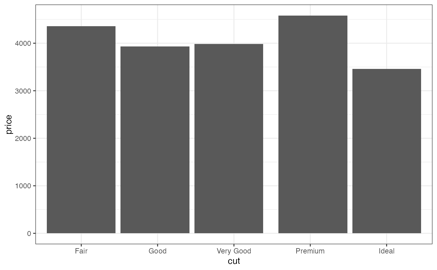
 gf_col(price ~ cut, data = diamonds, stat = "summary_bin", fun.y = "mean")
#> No summary function supplied, defaulting to `mean_se()`
gf_col(price ~ cut, data = diamonds, stat = "summary_bin", fun.y = "mean")
#> No summary function supplied, defaulting to `mean_se()`
 # Don't use gf_lims() to zoom into a summary plot - this throws the
# data away
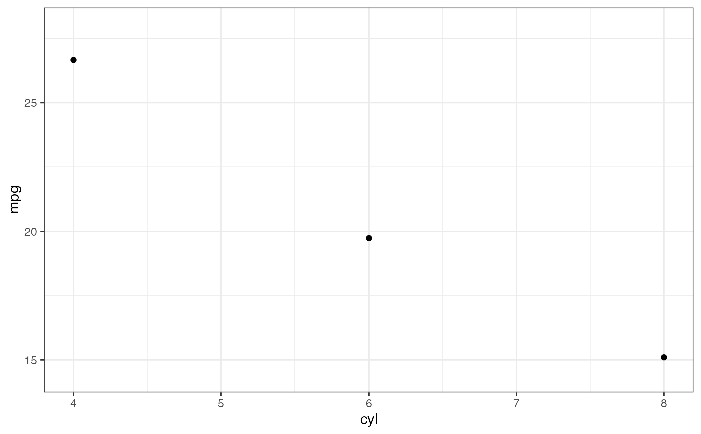
p <- gf_summary(mpg ~ cyl, data = mtcars, fun.y = "mean", geom = "point")
p
#> No summary function supplied, defaulting to `mean_se()`
# Don't use gf_lims() to zoom into a summary plot - this throws the
# data away
p <- gf_summary(mpg ~ cyl, data = mtcars, fun.y = "mean", geom = "point")
p
#> No summary function supplied, defaulting to `mean_se()`
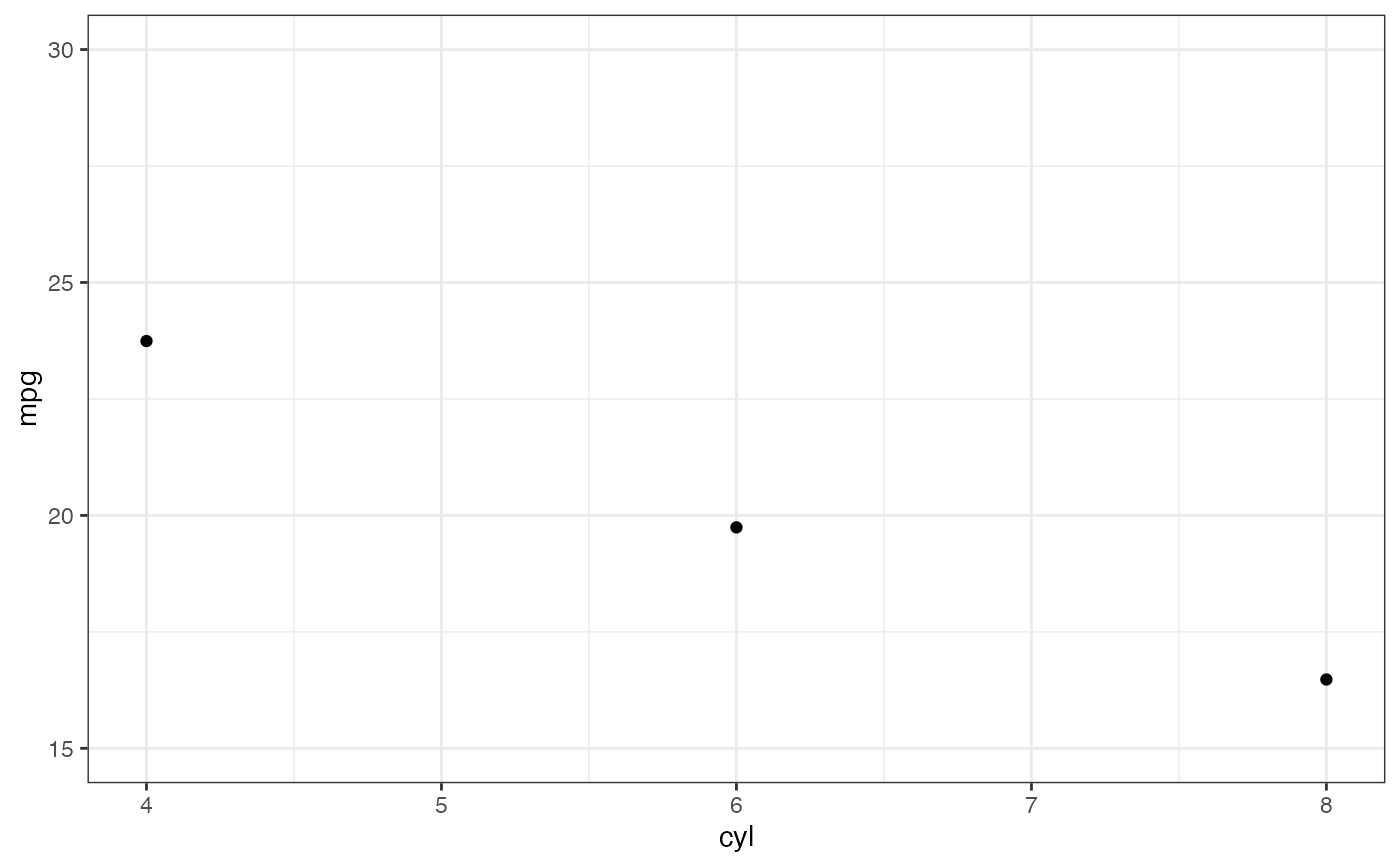
 p |> gf_lims(y = c(15, 30))
#> No summary function supplied, defaulting to `mean_se()`
#> Warning: Removed 9 rows containing non-finite outside the scale range
#> (`stat_summary()`).
p |> gf_lims(y = c(15, 30))
#> No summary function supplied, defaulting to `mean_se()`
#> Warning: Removed 9 rows containing non-finite outside the scale range
#> (`stat_summary()`).
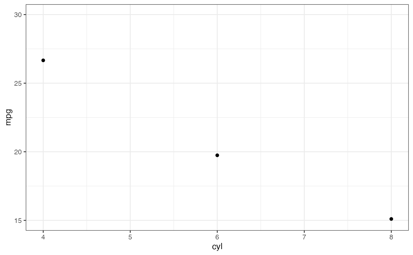
 # Instead use coord_cartesian()
p |> gf_refine(coord_cartesian(ylim = c(15, 30)))
#> No summary function supplied, defaulting to `mean_se()`
# Instead use coord_cartesian()
p |> gf_refine(coord_cartesian(ylim = c(15, 30)))
#> No summary function supplied, defaulting to `mean_se()`
 # A set of useful summary functions is provided from the Hmisc package.
if (FALSE) { # \dontrun{
p <- gf_jitter(mpg ~ cyl, data = mtcars, width = 0.15, height = 0); p
p |> gf_summary(fun.data = mean_cl_boot, color = "red")
p |> gf_summary(fun.data = mean_cl_boot, color = "red", geom = "crossbar")
p |> gf_summary(fun.data = mean_sdl, group = ~ cyl, color = "red",
geom = "crossbar", width = 0.3)
p |> gf_summary(group = ~ cyl, color = "red", geom = "crossbar", width = 0.3,
fun.data = mean_sdl, fun.args = list(mult = 1))
p |> gf_summary(fun.data = median_hilow, group = ~ cyl, color = "red",
geom = "crossbar", width = 0.3)
} # }
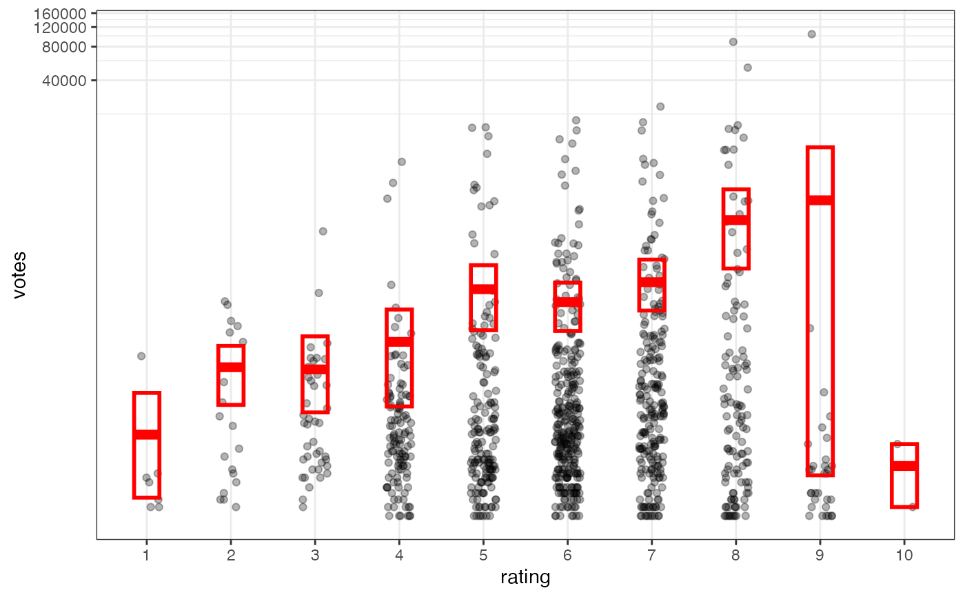
# An example with highly skewed distributions:
if (require("ggplot2movies")) {
set.seed(596)
Mov <- movies[sample(nrow(movies), 1000), ]
m2 <- gf_jitter(votes ~ factor(round(rating)), data = Mov, width = 0.15, height = 0, alpha = 0.3)
m2 <- m2 |>
gf_summary(fun.data = "mean_cl_boot", geom = "crossbar",
colour = "red", width = 0.3) |>
gf_labs(x = "rating")
m2
# Notice how the overplotting skews off visual perception of the mean
# supplementing the raw data with summary statistics is _very_ important
# Next, we'll look at votes on a log scale.
# Transforming the scale means the data are transformed
# first, after which statistics are computed:
m2 |> gf_refine(scale_y_log10())
# Transforming the coordinate system occurs after the
# statistic has been computed. This means we're calculating the summary on the raw data
# and stretching the geoms onto the log scale. Compare the widths of the
# standard errors.
m2 |> gf_refine(coord_trans(y="log10"))
}
#> Loading required package: ggplot2movies
#> Warning: `coord_trans()` was deprecated in ggplot2 4.0.0.
#> ℹ Please use `coord_transform()` instead.
# A set of useful summary functions is provided from the Hmisc package.
if (FALSE) { # \dontrun{
p <- gf_jitter(mpg ~ cyl, data = mtcars, width = 0.15, height = 0); p
p |> gf_summary(fun.data = mean_cl_boot, color = "red")
p |> gf_summary(fun.data = mean_cl_boot, color = "red", geom = "crossbar")
p |> gf_summary(fun.data = mean_sdl, group = ~ cyl, color = "red",
geom = "crossbar", width = 0.3)
p |> gf_summary(group = ~ cyl, color = "red", geom = "crossbar", width = 0.3,
fun.data = mean_sdl, fun.args = list(mult = 1))
p |> gf_summary(fun.data = median_hilow, group = ~ cyl, color = "red",
geom = "crossbar", width = 0.3)
} # }
# An example with highly skewed distributions:
if (require("ggplot2movies")) {
set.seed(596)
Mov <- movies[sample(nrow(movies), 1000), ]
m2 <- gf_jitter(votes ~ factor(round(rating)), data = Mov, width = 0.15, height = 0, alpha = 0.3)
m2 <- m2 |>
gf_summary(fun.data = "mean_cl_boot", geom = "crossbar",
colour = "red", width = 0.3) |>
gf_labs(x = "rating")
m2
# Notice how the overplotting skews off visual perception of the mean
# supplementing the raw data with summary statistics is _very_ important
# Next, we'll look at votes on a log scale.
# Transforming the scale means the data are transformed
# first, after which statistics are computed:
m2 |> gf_refine(scale_y_log10())
# Transforming the coordinate system occurs after the
# statistic has been computed. This means we're calculating the summary on the raw data
# and stretching the geoms onto the log scale. Compare the widths of the
# standard errors.
m2 |> gf_refine(coord_trans(y="log10"))
}
#> Loading required package: ggplot2movies
#> Warning: `coord_trans()` was deprecated in ggplot2 4.0.0.
#> ℹ Please use `coord_transform()` instead.