Chapter 1 Introduction

Modern statistics is done on the computer. There was a time, 60 years ago and before, when computation could only be done by hand or using balky mechanical calculators. The methods of applied statistics developed during this time reflected what could be done using such calculators, not necessarily what was best for illuminating the system under study. These methods took on a life of their own — they became the operational definition of statistics. They continue to be taught today, using electronic calculators or personal computers or even just using paper and pencil. For the old statistical methods, computers are merely a labor saving device.

But not for modern statistics. The statistical methods at the core of this book cannot be applied in a authentic and realistic way without powerful computers. Thirty years ago, many of the methods could not be done at all unless you had access to the resources of a government agency or a large university. But with the revolutionary advances in computer hardware and numerical algorithms over the last half-century, modern statistical calculations can be performed on an ordinary home computer or laptop. (Even a cell phone has phenomenal computational power, often besting the mainframes of thirty years ago.) Hardware and software today pose no limitation; they are readily available.

Each chapter of this book includes a section on computational technique. Many readers will be completely new to the use of computers for scientific and statistial work, so the first chapters cover the foundations, techniques that are useful for many different aspects of computation. Working through the early chapters is essential for developing the skills that will be used later in actual statistical work. It will take a few hours, but this investment will pay off handsomely.

Chances are, you use a computer almost every day: for email, word-processing, managing your music or your photograph collection, perhaps even using a spreadsheet program for accounting. The software you use for such activities makes it easy to get started. Possibly you have never even looked at an instruction manual or used the “help” features on your computer.

When you use a word processor or email, the bulk of what you enter into the computer — the content of your documents and email — is without meaning to the computer. This is not at all to say that it is meaningless. Your documents and letters are intended for human readers; most of the work you do is directed so that the recipients can understand them. But the computer doesn’t need to understand what you write in order to format it, print it, or transmit it over the Internet.

When doing scientific and statistical computing, things are different. What you enter into the computer is instructions to the computer to perform calculations and re-arrangements of data. Those instructions have to be comprehensible to the computer. If they make no sense or if they are inconsistent or ill formed, the computer won’t be able to carry out your instructions. Worse, if the instructions make sense in some formal way but don’t convey your actual intentions, the computer will perform some operation but the result will mislead you.

The difficulty with using software for mathematics and statistics is in making sure that your instructions make sense and do what you want them to do. This difficulty is not a matter of bad software design; it’s intrinsic to the problem of communicating your intentions to the computer. The same difficulty would arise in word processing if the computer had to make sense of your writing, rejecting it when a claim is unconvincing or when a sentence is ambiguous. Statistical computing pioneer John Chambers refers to the “Prime Directive” of software (???): “to program in such a way that computations can be understood and trusted.”

Much of the design of software for scientific and statistical work is oriented around the difficulty of communicating intentions. A popular approach is based on the computer mouse: the program provides a list of possible operations — like the keys on a calculator — and lets the user choose which operation to apply to some selected data. This style of user interface is employed, for example, in spreadsheet software, letting users add up columns of numbers, make graphs, etc. The reason this style is popular is that it can make things extremely easy … so long as the operation that you want has been included in the software. But things get very hard if you need to construct your own operation and it can be difficult to understand or trust the operations performed by others.

Another style of scientific computation — the one used in this book — is based on language. Rather than selecting an option with a mouse, you construct a command that conveys both the operation that you want and the data to which you want to apply that operation. There are dramatic advantages to this language-based style of computation:

It lets you connect computations to one another, so that the output of one operation can become the input to another.
It lets you repeat the operation on new or modified data, allowing you to automate tedious tasks and, importantly, to verify the correctness of your computations on data where you already know the answer.
It lets you accumulate the results of previous operations, treating those results as new data.
It lets you document concisely what was done so that you can demonstrate that what you said you did is what you actually did. In this way, you or others can repeat the analysis later if necessary to confirm your results.
It lets you modify the computation in a controlled way to correct it or to vary some aspect of it while holding other aspects exactly the same as in the original.

In order to use the language-based approach, you will need to learn a few principles of the language itself: some vocabulary, some syntax, some grammar. This is much, much easier for the computer language than for a natural language like English or Chinese; it will take you only a couple of hours before you are fluent enough to do useful computations. In addition to letting you perform scientific computations in ways that use the computer and your own time and effort effectively, the principles that you will learn are broadly applicable to many computer systems and can provide significant insight even to how to use mouse-based interfaces.

1.1 The Choice of Software

The software package used in this book is called R. The R package provides an environment for doing statistical and scientific computation at a professional level. It was designed for statistics work, but suitable for other forms of scientific calculations and the creation of high-quality scientific graphics.

There are several other major software packages widely used in statistics. Among the leaders are SPSS, SAS, and Stata. Each of them provides the computational power needed for statistical modeling. Each has its own advantages and its own devoted group of users.

One reason for the choice of R is that it offers a command-based computing environment. That makes it much easier to write about computing and also reveals better the structure of the computing process. (???) R is available for free and works on the major types of computers, e.g., Windows, Macintosh, and Unix/Linux. The RStudio software lets you work with a complete R system using an ordinary web browser or on your own computer.

In making your own choice, the most important thing is this: choose something! Readers who are familiar with SPSS, SAS, or STATA can use the information in each chapter’s computational technique section to help them identify the facilities to look for in those packages.

Another form of software that’s often used with data is the spreadsheet. Examples are Excel and Google Spreadsheets. Spreadsheets are effective for entering data and have nice facilities for formatting tables. The visual layout of the data seems to be intuitive to many people. Many businesses use spreadsheets and they are widely taught in high schools. Unfortunately, they are very difficult to use for statistical analyses of any sophistication. Indeed, even some very elementary statistical tasks such as making a histogram are difficult with spreadsheets and the results are usually unsatisfactory from a graphical point of view. Worse, spreadsheets can be very hard to use reliably. There are lots of opportunities to make mistakes that will go undetected. As a result, despite the popularity of spreadsheets, I encourage you to reserve them for data entry and consider other software for the analysis of your data.

1.2 The R Command Console

Depending on your circumstances, you may prefer to install R as software on your own computer, or use a web-based (“cloud computing”) service such as RStudio that runs through a web browser.
If you are using this book with a course, your instructor may have set up a system for you. If you are on your own, follow the set-up instructions available on-line at .

Depending on whether you run R on your own computer or in the cloud, you will start R either by clicking on an icon in the familiar way or by logging in to the web service. In either case, you will see a console panel in which you will be typing your commands to R. It will look something like Figure ??.¹

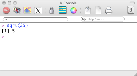
Figure 1.1: The R command console.

The R console gives you great power to carry out statistical and other mathematical and scientific operations. To use this power, you need to learn a little bit about the syntax and meaning of R commands. Once you have learned this, operations become simple to perform.

1.3 Invoking an Operation

People often think of computers as doing things: sending email, playing music, storing files. Your job in using a computer is to tell the computer what to do. There are many different words used to refer to the “what”: a procedure, a task, a function, a routine, and so on. I’ll use the word computation. Admittedly, this is a bit circular, but it is easy to remember: computers perform computations.

Complex computations are built up from simpler computations. This may seem obvious, but it is a powerful idea. An algorithm is just a description of a computation in terms of other computations that you already know how to perform. To help distinguish between the computation as a whole and the simpler parts, it is helpful to introduce a new word: an operator (??? software!operator) performs a computation.

It’s helpful to think of the computation carried out by an operator as involving four parts:

The name of the operator
The input arguments
The output value
Side effects A typical operation takes one or more input arguments and uses the information in these to produce an output value. Along the way, the computer might take some action: display a graph, store a file, make a sound, etc. These actions are called side effects.

To tell the computer to perform a computation — call this invoking an operation or giving a command — you need to provide the name and the input arguments in a specific format. The computer then returns the output value. For example, the command sqrt(25) invokes the square root operator (named sqrt) on the argument 25. The output from the computation will, of course, be 5.

The syntax for invoking an operation consists of the operator’s name, followed by round parentheses. The input arguments go inside the parentheses.

The software program that you use to invoke operators is called an interpreter. (The interpreter is the program you are running when you start R.) You enter your commands as a dialog between you and the interpreter. To start, the interpreter prints a prompt, after which you type your command:

When you press “Enter,” the interpreter reads your command and performs the computation. For commands such as this one, the interpreter will print the output value from the computation:

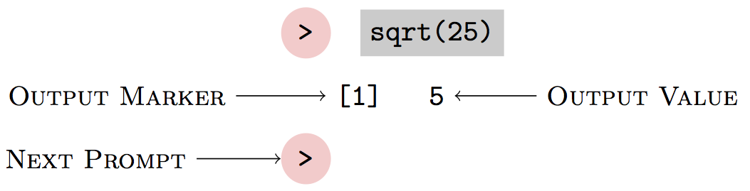
The dialog continues as the interpreter prints another prompt and waits for your further command.

To save space, I’ll usually show just the give-and-take from one round of the dialog:

sqrt(25)

## [1] 5

(Go ahead! Type sqrt(25) after the prompt in the R interpreter, press ``enter,’’ and see what happens.)

Often, operations involve more than one argument. The various arguments are separated by commas. For example, here is an operation named seq

that produces a sequence of numbers:

seq(3,10)

## [1]  3  4  5  6  7  8  9 10

The first argument tells where to start the sequence, the second tells where to end it.

The order of the arguments is important. Here is the sequence produced when 10 is the first argument and 3 the second:

seq(10,3)

## [1] 10  9  8  7  6  5  4  3

For some operators, particularly those that have many input arguments, some of the arguments can be referred to by name rather than position. This is particularly useful when the named argument has a sensible default value. For example, the seq operator can be instructed how big a jump to take between successive items in the sequence. This is accomplished using an argument named by:

seq(3,10,by=2)

## [1] 3 5 7 9

Depending on the circumstances, all four parts of a operation need not be present. For example, the date

operation returns the current time and date; no input arguments are needed.

date()

## [1] "Sat Sep  3 12:12:16 2016"

Note that even though there are no arguments, the parentheses are still used. Think of the pair of parentheses as meaning, “Do this.”

1.3.1 Naming and Storing Values

Often the value returned by an operation will be used later on. Values can be stored for later use with the assignment operator . This has a different syntax that reminds the user that a value is being stored. Here’s an example of a simple assignment:

x <- 16

This command has stored the value 16 under the name x. The syntax is always the same: an equal sign (=) with a name on the left and a value on the right.

Such stored values are called objects . Making an assignment to an object defines the object. Once an object has been defined, it can be referred to and used in later computations.

Notice that an assignment operation does not return a value or display a value. Its sole purpose is to have the side effects of defining the object and thereby storing a value under the object’s name.

To refer to the value stored in the object, just use the object’s name itself. For instance:

## [1] 16

Doing a computation on the value stored in an object is much the same: <<>>= sqrt(x) @

You can create as many objects as you like and give them names that remind you of their purpose. Some examples: wilma, ages, temp, dog.houses, foo3. There are some rules for object names:

Use only letters and numbers and the two punctuation marks “dot” (.) and “underscore” (_).
Do NOT use spaces anywhere in the name.
A number or underscore cannot be the first character in the name.
Capital letters are treated as distinct from lower-case letters. The objects named wilma and Wilma are different.
For the sake of readability, keep object names short. But if you really must have an object named something like agesOfChildrenFromTheClinicalTrial, feel free.

Objects can store all sorts of things, for example a sequence of numbers:

x <- seq(1,7)

When you assign a new value to an existing object, as just done to x, the former value of that object is erased from the computer memory. The former value of x was 16, but after the above assignment command it is

## [1] 1 2 3 4 5 6 7

The value of an object is changed only via the assignment operator. Using an object in a computation does not change the value. For example, suppose you invoke the square-root operator on x:

sqrt(x)

## [1] 1.000000 1.414214 1.732051 2.000000 2.236068 2.449490 2.645751

The square roots have been returned as a value, but this doesn’t change the value of x:

## [1] 1 2 3 4 5 6 7

If you want to change the value of x, you need to use the assignment operator:

x <- sqrt(x)
x

## [1] 1.000000 1.414214 1.732051 2.000000 2.236068 2.449490 2.645751

1.3.2 Assignment vs Algebra

An assignment command like x = sqrt(x) can be confusing to people who are used to algebraic notation. In algebra, the equal sign describes a relationship between the left and right sides.
So, \(x = \sqrt{x}\) tells us about how the quantity \(x\) and the quantity \(\sqrt{x}\) are related. Students are usually trained to “solve” such relationships, going through a series of algebraic steps to find values for \(x\) that are consistent with the mathematical statement. (For \(x = \sqrt{x}\), the solutions are \(x=0\) and \(x=1\).) In contrast, the assignment command x = sqrt(x) is a way of replacing the previous values stored in x with new values that are the square root of the old ones.

1.3.3 Connecting Computations

The brilliant thing about organizing operators in terms of input arguments and output values is that the output of one operator can be used as an input to another. This lets complicated computations be built out of simpler ones.

For example, suppose you have a list of 10000 voters in a precinct and you want to select a random sample of 20 of them for a survey. The seq operator can be used to generate a set of 10000 choices. The sample operator can be used to select some of these choices at random.

One way to connect the computations is by using objects to store the intermediate outputs.

choices = seq(1,10000)
sample( choices, 20 )

##  [1] 9831 9797 9845 4901 4270 7064 2983 9339 5801 9553  111 7027 3502 3423
## [15] 6580 9858 9232  938  204 6090

You can also pass the output of an operator directly as an argument to another operator. Here’s another way to accomplish exactly the same thing as the above.

sample( seq(1,10000), 20 )

##  [1] 6228 4446 7432 4398 2591 7417 3058 7853  872 4528 2149 5138 9200 5532
## [15] 7369 1582 4311 4098 1675 9577

1.3.4 Numbers and Arithmetic

The language has a concise notation for arithmetic that looks very much like the traditional one:

7+2

## [1] 9

3*4

## [1] 12

5/2

## [1] 2.5

3-8

## [1] -5

-3

## [1] -3

5^2

## [1] 25

Arithmetic operators, like any other operators, can be connected to form more complicated computations. For instance,

8+4/2

## [1] 10

To a human reader, the command 8+4/2 might seem ambiguous. Is it intended to be (8+4)/2 or 8+(4/2)? The computer uses unambiguous rules to interpret the expression, but it’s a good idea for you to use parethesis so that you can make sure that what you intend is what the computer carries out:

(8+4)/2

## [1] 6

Traditional mathematical notation uses superscripts and radicals to indicate exponentials and roots, e.g., \(3^2\) or \(\sqrt{3}\) or \(\sqrt[3]{8}\). This special typography doesn’t work well with an ordinary keyboard, so R and most other computer languages uses a different notation:

3^2

## [1] 9

sqrt(3)

## [1] 1.732051

8^(1/3)

## [1] 2

There is a large set of mathematical functions: exponentials, logs, trigonometric and inverse trigonometric functions, etc. Some examples:

Traditional	Computer
\(e^2\)	`exp(2)`
\(\log_e(100)\)	`log(100)`
\(\log_{10}(100)\)	`log10(100)`
\(\log_{2}(100)\)	`log2(100)`
\(\cos( \frac{\pi}{2})\)	`cos(pi/2)`
\(\sin( \frac{\pi}{2})\)	`sin(pi/2)`
\(\tan( \frac{\pi}{2})\)	`tan(pi/2)`
\(\cos^{-1}(-1)\)	`acos(-1)`

Numbers can be written in scientific notation. For example, the “universal gravitational constant” that describes the gravitational attraction between masses is \(6.67428 \times 10^{-11}\) (with units meters-cubed per kilogram per second squared). In the computer notation, this would be written G=6.67428e-11. The Avogradro constant, which gives the number of atoms in a mole, is \(6.02214179 \times 10^{23}\) per mole, or 6.02214178e23.

The computer language does not directly support the recording of units. This is unfortunate, since in the real world numbers often have units and the units matter. For example, in 1999 the Mars Climate Orbiter crashed into Mars because the design engineers specified the engine’s thrust in units of pounds, while the guidance engineers thought the units were newtons.

Computer arithmetic is accurate and reliable, but it often involves very slight rounding of numbers. Ordinarily, this is not noticeable. However, it can become apparent in some calculations that produce results that are zero. For example, mathematically \(\sin(\pi) = 0\), however the computer does not duplicate this mathematical relationship exactly:

sin(pi)

## [1] 1.224647e-16

Whether a number like this is properly interpreted as “close to zero,” depends on the context and, for quantities that have units, on the units themselves. For instance, the unit “parsec” is used in astronomy in reporting distances between stars. The closest star to the sun is Proxima, at a distance of 1.3 parsecs.² A distance of \(1.22 \times 10^{-16}\) parsecs is tiny in astronomy but translates to about 2.5 meters — not so small on the human scale.

In statistics, many calculations relate to probabilities which are always in the range 0 to 1. On this scale, 1.22e-16 is very close to zero.

There are two “special” numbers. Inf stands for \(\infty\), as in

1/0

## [1] Inf

NaN stands for “not a number,” and is the result when a numerical operation isn’t defined, for instance

0/0

## [1] NaN

1.3.5 Aside: Complex numbers

Mathematically oriented readers will wonder why R should have any trouble with a computation like \(\sqrt{-9}\); the result is the imaginary number \(3i\). R works with complex numbers, but you have to tell the system that this is what you want to do. To calculate \(\sqrt{-9}\), use .

1.3.6 Types of Objects

Most of the examples used so far have dealt with numbers. But computers work with other kinds of information as well: text, photographs, sounds, sets of data, and so on. The word type is used to refer to the kind of information.

Modern computer languages support a great variety of types.
It’s important to know about the types of data because operators expect their input arguments to be of specific types. When you use the wrong type of input, the computer might not be able process your command.

For the purpose of starting with R, it’s important to distinguish among three basic types:

numeric The numbers of the sort already encountered.
data frames Collections of data more or less in the form of a spreadsheet table. The Computation Technique section in Chapter @ref(“chap:data-cases-variables”) introduces the operators for working with data frames.
character Text data.

You indicate character data to the computer by enclosing the text in double quotation marks. For example:

filename = "swimmers.csv"

There is something a bit subtle going on in the above command, so look at it carefully. The purpose of the command is to create an object, named filename, that stores a little bit of text data. Notice that the name of the object is not put in quotes, but the text characters are.

Whenever you refer to an object name, make sure that you don’t use quotes, for example:

filename

## [1] "swimmers.csv"

If you make a command with the object name in quotes, it won’t be treated as referring to an object. Instead, it will merely mean the text itself:

"filename"

## [1] "filename"

Similarly, if you omit the quotation marks from around text, the computer will treat it as if it were an object name and will look for the object of that name. For instance, the following command directs the computer to look up the value contained in an object named swimmers.csv and insert that value into the object filename.

filename <- swimmers.csv

## Error in eval(expr, envir, enclos): object 'swimmers.csv' not found

As it happens, there was no object named swimmers.csv because it had not been defined by any previous assignment command. So, the computer generated an error.

For the most part, you will not need to use very many operators on text data; you just need to remember to include text, such as file names, in quotation marks, "like this".

DRAFT: Look how out of date this is! No notion of RStudio. Do note that in the knitr chunk, the chunk label (“console-picture”) becomes part of the label for the picture, which can be put in with \@ref(console-picture) as in Figure ??.↩
News from August 2016: Astronomers have announced that Proxima has a planet orbiting it in the “habitable zone.”↩