These functions create layers that display lines described i various ways. Unlike most
of the plotting functions in ggformula, these functions do not take a formula
as input for describing positional attributes of the plot.
Usage
gf_abline(
  object = NULL,
  gformula = NULL,
  data = NULL,
  ...,
  slope,
  intercept,
  color,
  linetype,
  linewidth,
  alpha,
  xlab,
  ylab,
  title,
  subtitle,
  caption,
  show.legend = NA,
  show.help = NULL,
  inherit = FALSE,
  environment = parent.frame()
)

gf_hline(
  object = NULL,
  gformula = NULL,
  data = NULL,
  ...,
  yintercept,
  color,
  linetype,
  linewidth,
  alpha,
  xlab,
  ylab,
  title,
  subtitle,
  caption,
  position = "identity",
  show.legend = NA,
  show.help = NULL,
  inherit = FALSE,
  environment = parent.frame()
)

gf_vline(
  object = NULL,
  gformula = NULL,
  data = NULL,
  ...,
  xintercept,
  color,
  linetype,
  linewidth,
  alpha,
  xlab,
  ylab,
  title,
  subtitle,
  caption,
  position = "identity",
  show.legend = NA,
  show.help = NULL,
  inherit = FALSE,
  environment = parent.frame()
)

gf_coefline(object = NULL, coef = NULL, model = NULL, ...)
Arguments
- object
When chaining, this holds an object produced in the earlier portions of the chain. Most users can safely ignore this argument. See details and examples.
- gformula
Must be
NULL.- data
The data to be displayed in this layer. There are three options:
If
NULL, the default, the data is inherited from the plot data as specified in the call toggplot().A
data.frame, or other object, will override the plot data. All objects will be fortified to produce a data frame. Seefortify()for which variables will be created.A
functionwill be called with a single argument, the plot data. The return value must be adata.frame, and will be used as the layer data. Afunctioncan be created from aformula(e.g.~ head(.x, 10)).- ...
Additional arguments. Typically these are (a) ggplot2 aesthetics to be set with
attribute = value, (b) ggplot2 aesthetics to be mapped withattribute = ~ expression, or (c) attributes of the layer as a whole, which are set withattribute = value.- color
A color or a formula used for mapping color.
- linetype
A linetype (numeric or "dashed", "dotted", etc.) or a formula used for mapping linetype.
- linewidth
A numerical line width or a formula used for mapping linewidth.
- alpha
Opacity (0 = invisible, 1 = opaque).
- xlab
Label for x-axis. See also
gf_labs().- ylab
Label for y-axis. See also
gf_labs().- title, subtitle, caption
Title, sub-title, and caption for the plot. See also
gf_labs().- show.legend
logical. Should this layer be included in the legends?
NA, the default, includes if any aesthetics are mapped.FALSEnever includes, andTRUEalways includes. It can also be a named logical vector to finely select the aesthetics to display. To include legend keys for all levels, even when no data exists, useTRUE. IfNA, all levels are shown in legend, but unobserved levels are omitted.- show.help
If
TRUE, display some minimal help.- inherit
A logical indicating whether default attributes are inherited.
- environment
An environment in which to look for variables not found in
data.- position
A position adjustment to use on the data for this layer. This can be used in various ways, including to prevent overplotting and improving the display. The
positionargument accepts the following:The result of calling a position function, such as
position_jitter(). This method allows for passing extra arguments to the position.A string naming the position adjustment. To give the position as a string, strip the function name of the
position_prefix. For example, to useposition_jitter(), give the position as"jitter".For more information and other ways to specify the position, see the layer position documentation.
- xintercept, yintercept, slope, intercept
Parameters that control the position of the line. If these are set,
data,mappingandshow.legendare overridden.- coef
A numeric vector of coefficients.
- model
A model from which to extract coefficients.
Examples
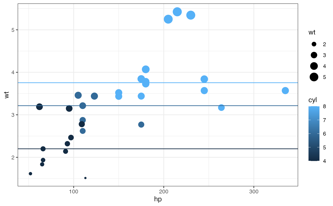
mtcars2 <- df_stats(wt ~ cyl, data = mtcars, median_wt = median)
gf_point(wt ~ hp, size = ~wt, color = ~cyl, data = mtcars) |>
gf_abline(slope = ~0, intercept = ~median_wt, color = ~cyl, data = mtcars2)
 gf_point(wt ~ hp, size = ~wt, color = ~cyl, data = mtcars) |>
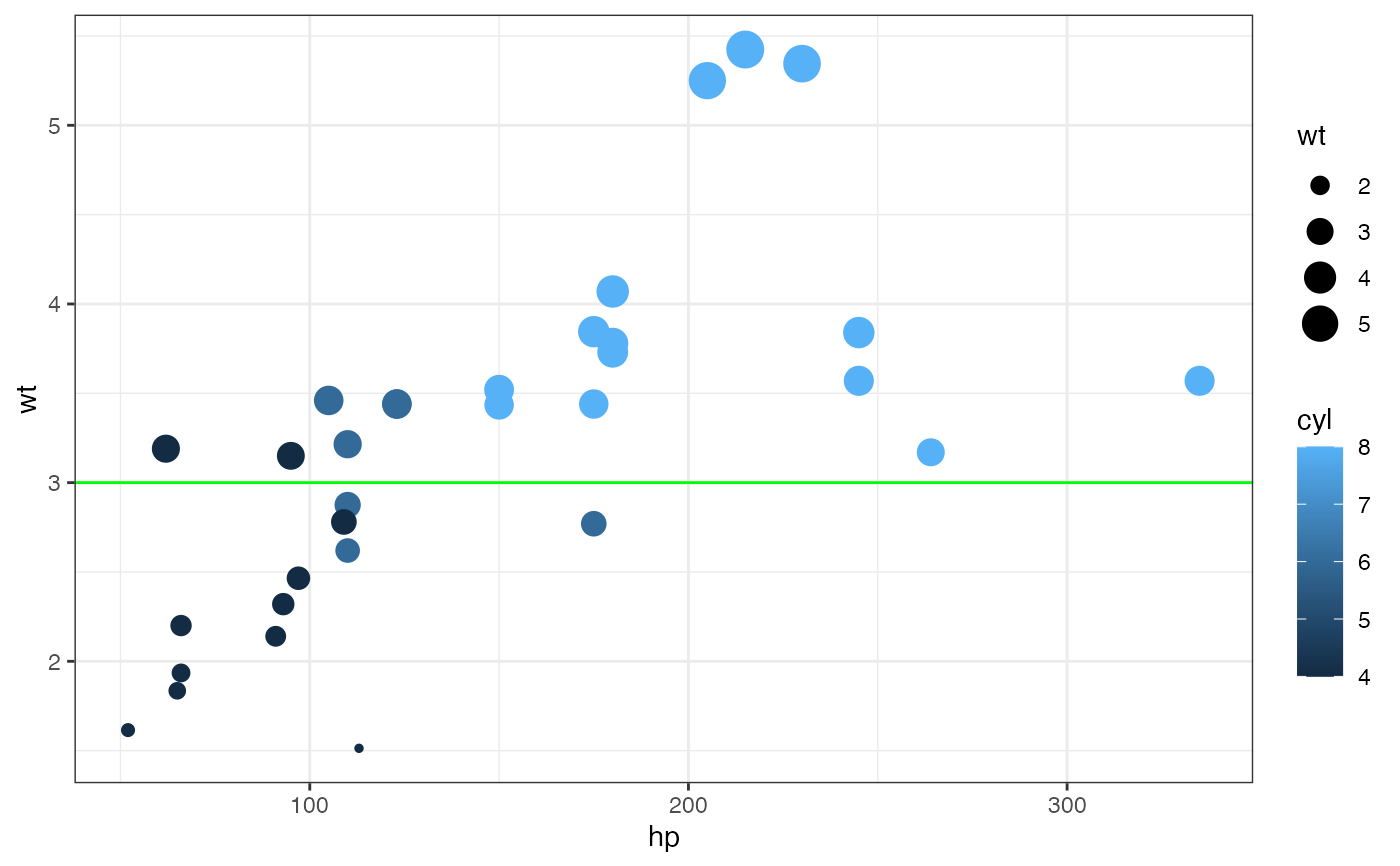
gf_abline(slope = 0, intercept = 3, color = "green")
gf_point(wt ~ hp, size = ~wt, color = ~cyl, data = mtcars) |>
gf_abline(slope = 0, intercept = 3, color = "green")
 # avoid warnings by using formulas:
gf_point(wt ~ hp, size = ~wt, color = ~cyl, data = mtcars) |>
gf_abline(slope = ~0, intercept = ~3, color = "green")
# avoid warnings by using formulas:
gf_point(wt ~ hp, size = ~wt, color = ~cyl, data = mtcars) |>
gf_abline(slope = ~0, intercept = ~3, color = "green")
 gf_point(wt ~ hp, size = ~wt, color = ~cyl, data = mtcars) |>
gf_hline(yintercept = ~median_wt, color = ~cyl, data = mtcars2)
gf_point(wt ~ hp, size = ~wt, color = ~cyl, data = mtcars) |>
gf_hline(yintercept = ~median_wt, color = ~cyl, data = mtcars2)
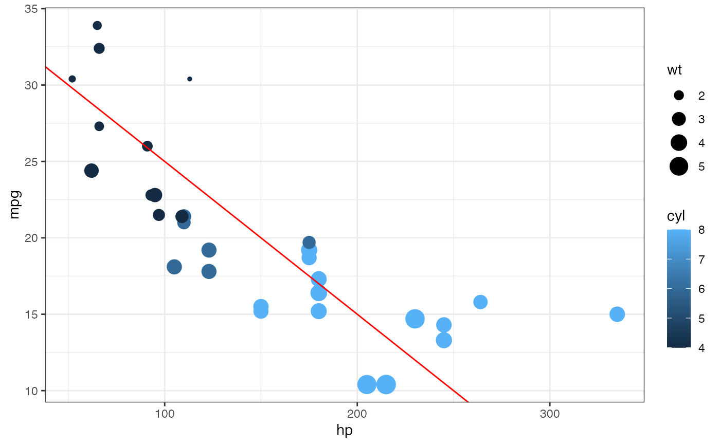
 gf_point(mpg ~ hp, color = ~cyl, size = ~wt, data = mtcars) |>
gf_abline(color = "red", slope = ~ - 0.10, intercept = ~ 35)
gf_point(mpg ~ hp, color = ~cyl, size = ~wt, data = mtcars) |>
gf_abline(color = "red", slope = ~ - 0.10, intercept = ~ 35)
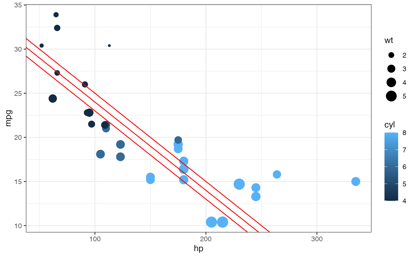
 gf_point(mpg ~ hp, color = ~cyl, size = ~wt, data = mtcars) |>
gf_abline(
color = "red", slope = ~slope, intercept = ~intercept,
data = data.frame(slope = -0.10, intercept = 33:35)
)
gf_point(mpg ~ hp, color = ~cyl, size = ~wt, data = mtcars) |>
gf_abline(
color = "red", slope = ~slope, intercept = ~intercept,
data = data.frame(slope = -0.10, intercept = 33:35)
)
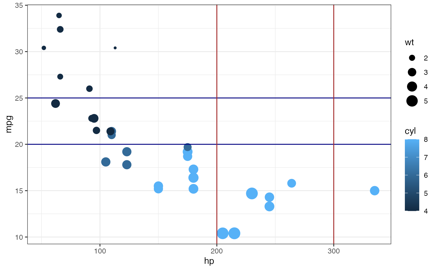
 # We can set the color of the guidelines while mapping color in other layers
gf_point(mpg ~ hp, color = ~cyl, size = ~ wt, data = mtcars) |>
gf_hline(color = "navy", yintercept = ~ c(20, 25), data = NA) |>
gf_vline(color = "brown", xintercept = ~ c(200, 300), data = NA)
#> Warning: `aes_string()` was deprecated in ggplot2 3.0.0.
#> ℹ Please use tidy evaluation idioms with `aes()`.
#> ℹ See also `vignette("ggplot2-in-packages")` for more information.
#> ℹ The deprecated feature was likely used in the ggformula package.
#> Please report the issue at
#> <https://github.com/ProjectMOSAIC/ggformula/issues>.
# We can set the color of the guidelines while mapping color in other layers
gf_point(mpg ~ hp, color = ~cyl, size = ~ wt, data = mtcars) |>
gf_hline(color = "navy", yintercept = ~ c(20, 25), data = NA) |>
gf_vline(color = "brown", xintercept = ~ c(200, 300), data = NA)
#> Warning: `aes_string()` was deprecated in ggplot2 3.0.0.
#> ℹ Please use tidy evaluation idioms with `aes()`.
#> ℹ See also `vignette("ggplot2-in-packages")` for more information.
#> ℹ The deprecated feature was likely used in the ggformula package.
#> Please report the issue at
#> <https://github.com/ProjectMOSAIC/ggformula/issues>.
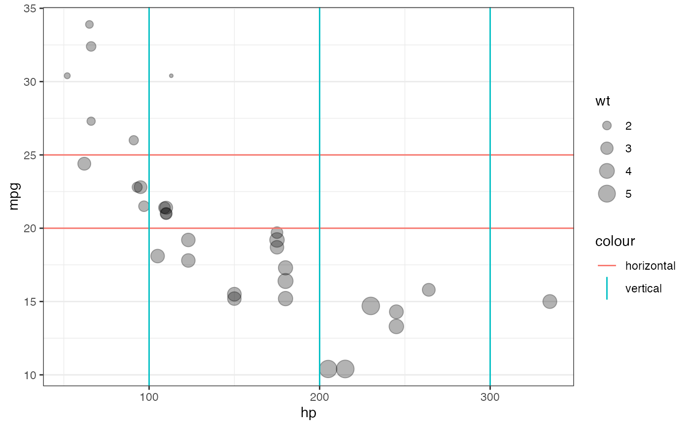
 # If we want to map the color of the guidelines, it must work with the
# scale of the other colors in the plot.
gf_point(mpg ~ hp, size = ~wt, data = mtcars, alpha = 0.3) |>
gf_hline(color = ~"horizontal", yintercept = ~ c(20, 25), data = NA) |>
gf_vline(color = ~"vertical", xintercept = ~ c(100, 200, 300), data = NA)
# If we want to map the color of the guidelines, it must work with the
# scale of the other colors in the plot.
gf_point(mpg ~ hp, size = ~wt, data = mtcars, alpha = 0.3) |>
gf_hline(color = ~"horizontal", yintercept = ~ c(20, 25), data = NA) |>
gf_vline(color = ~"vertical", xintercept = ~ c(100, 200, 300), data = NA)
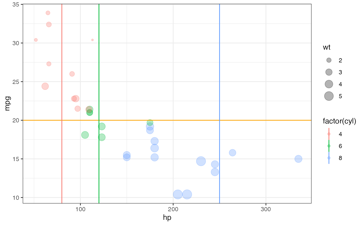
 gf_point(mpg ~ hp, size = ~wt, color = ~ factor(cyl), data = mtcars, alpha = 0.3) |>
gf_hline(color = "orange", yintercept = ~ 20) |>
gf_vline(color = ~ c("4", "6", "8"), xintercept = ~ c(80, 120, 250), data = NA)
gf_point(mpg ~ hp, size = ~wt, color = ~ factor(cyl), data = mtcars, alpha = 0.3) |>
gf_hline(color = "orange", yintercept = ~ 20) |>
gf_vline(color = ~ c("4", "6", "8"), xintercept = ~ c(80, 120, 250), data = NA)
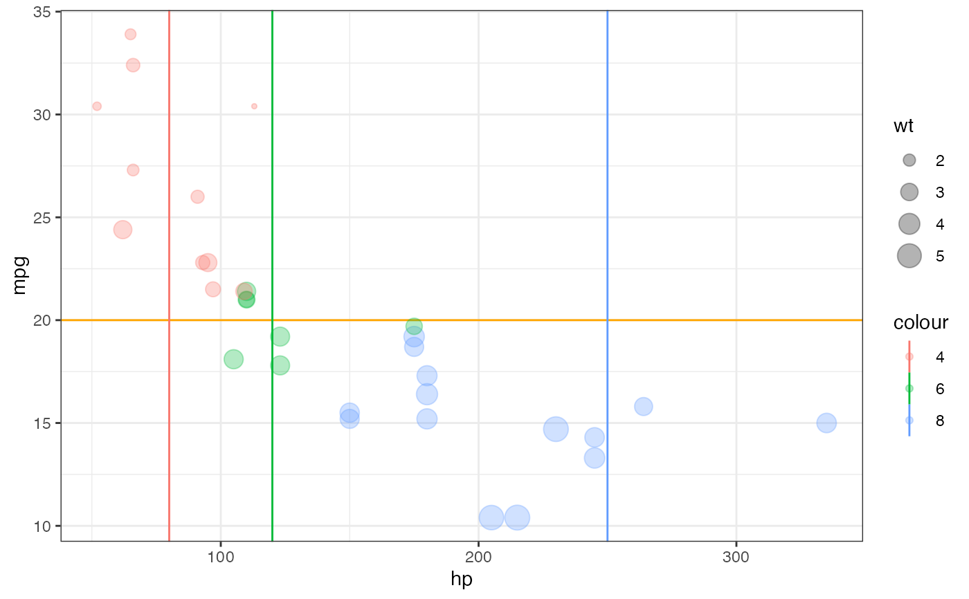
 gf_point(mpg ~ hp, size = ~wt, color = ~ factor(cyl), data = mtcars, alpha = 0.3) |>
gf_hline(color = "orange", yintercept = ~ 20) |>
gf_vline(color = c("green", "red", "blue"), xintercept = ~ c(80, 120, 250),
data = NA)
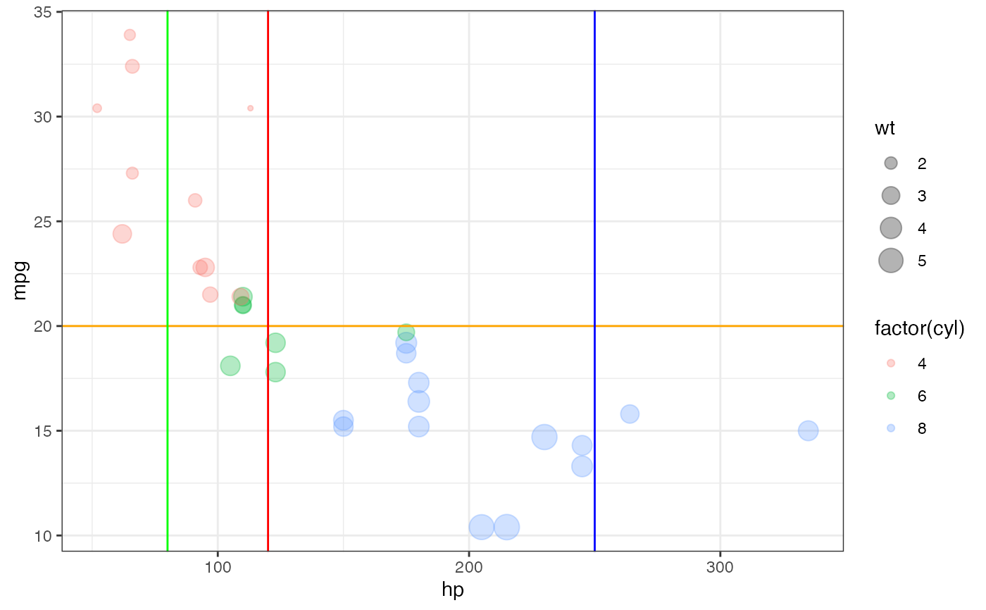
gf_point(mpg ~ hp, size = ~wt, color = ~ factor(cyl), data = mtcars, alpha = 0.3) |>
gf_hline(color = "orange", yintercept = ~ 20) |>
gf_vline(color = c("green", "red", "blue"), xintercept = ~ c(80, 120, 250),
data = NA)
 # reversing the layers requires using inherit = FALSE
gf_hline(color = "orange", yintercept = ~ 20) |>
gf_vline(color = ~ c("4", "6", "8"), xintercept = ~ c(80, 120, 250), data = NA) |>
gf_point(mpg ~ hp,
size = ~wt, color = ~ factor(cyl), data = mtcars, alpha = 0.3,
inherit = FALSE
)
# reversing the layers requires using inherit = FALSE
gf_hline(color = "orange", yintercept = ~ 20) |>
gf_vline(color = ~ c("4", "6", "8"), xintercept = ~ c(80, 120, 250), data = NA) |>
gf_point(mpg ~ hp,
size = ~wt, color = ~ factor(cyl), data = mtcars, alpha = 0.3,
inherit = FALSE
)