Plot distributions

Create a layer displaying a probability distribution.

Usage

gf_dist(
  object = ggplot(),
  dist,
  ...,
  xlim = NULL,
  kind = c("density", "cdf", "qq", "qqstep", "histogram"),
  resolution = 5000L,
  eps = 1e-06,
  params = NULL
)

Arguments

object

a gg object.

dist

A character string providing the name of a distribution. Any distribution for which the functions with names formed by prepending "d", "p", or "q" to dist exist can be used.

...

additional arguments passed both to the distribution functions and to the layer. Note: Possible ambiguities using params or by preceding plot argument with plot_.

xlim

A numeric vector of length 2 providing lower and upper bounds for the portion of the distribution that will be displayed. The default is to attempt to determine reasonable bounds using quantiles of the distribution.

kind

One of "density", "cdf", "qq", "qqstep", or "histogram" describing what kind of plot to create.

resolution

An integer specifying the number of points to use for creating the plot.

eps

a (small) numeric value. When other defaults are not available, the distribution is processed from the eps to 1 - eps quantiles.

params

a list of parameters for the distribution.

Examples

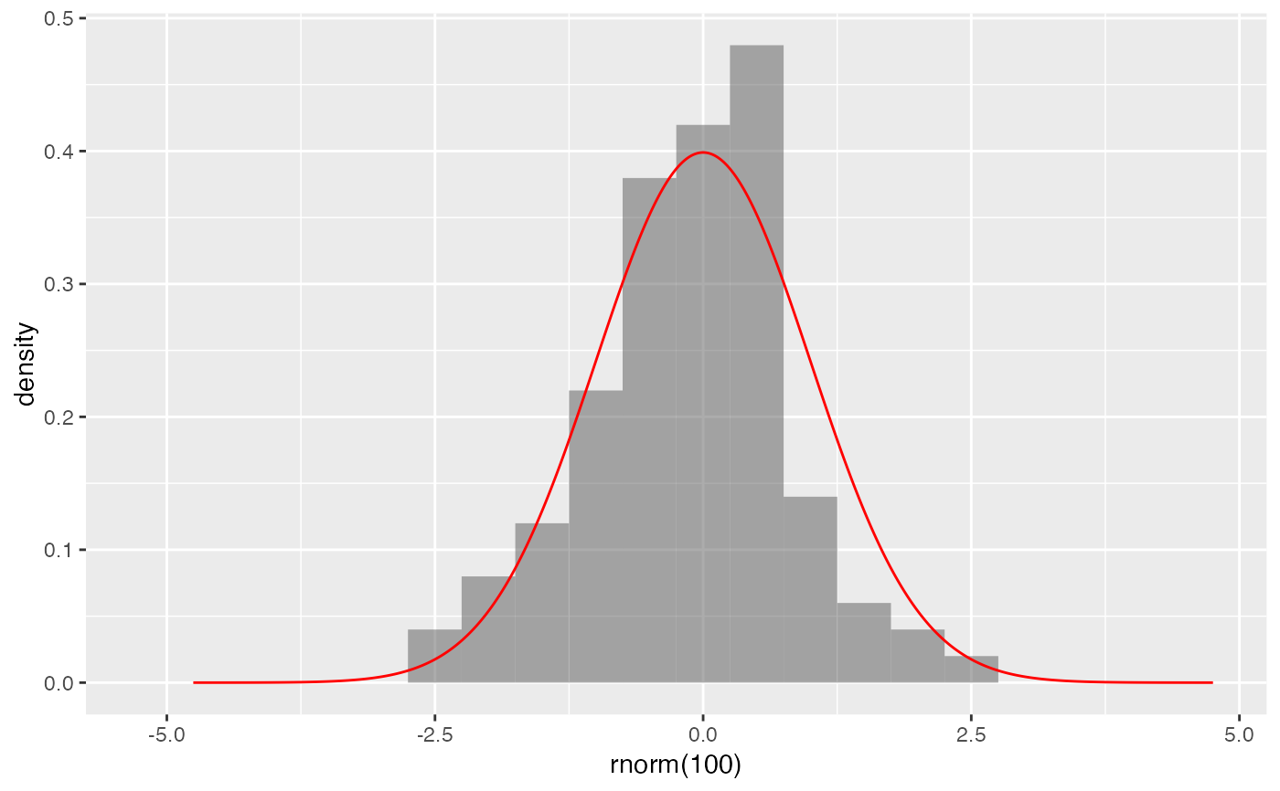
gf_dhistogram(~ rnorm(100), bins = 20) |>
  gf_dist("norm", color = "red")


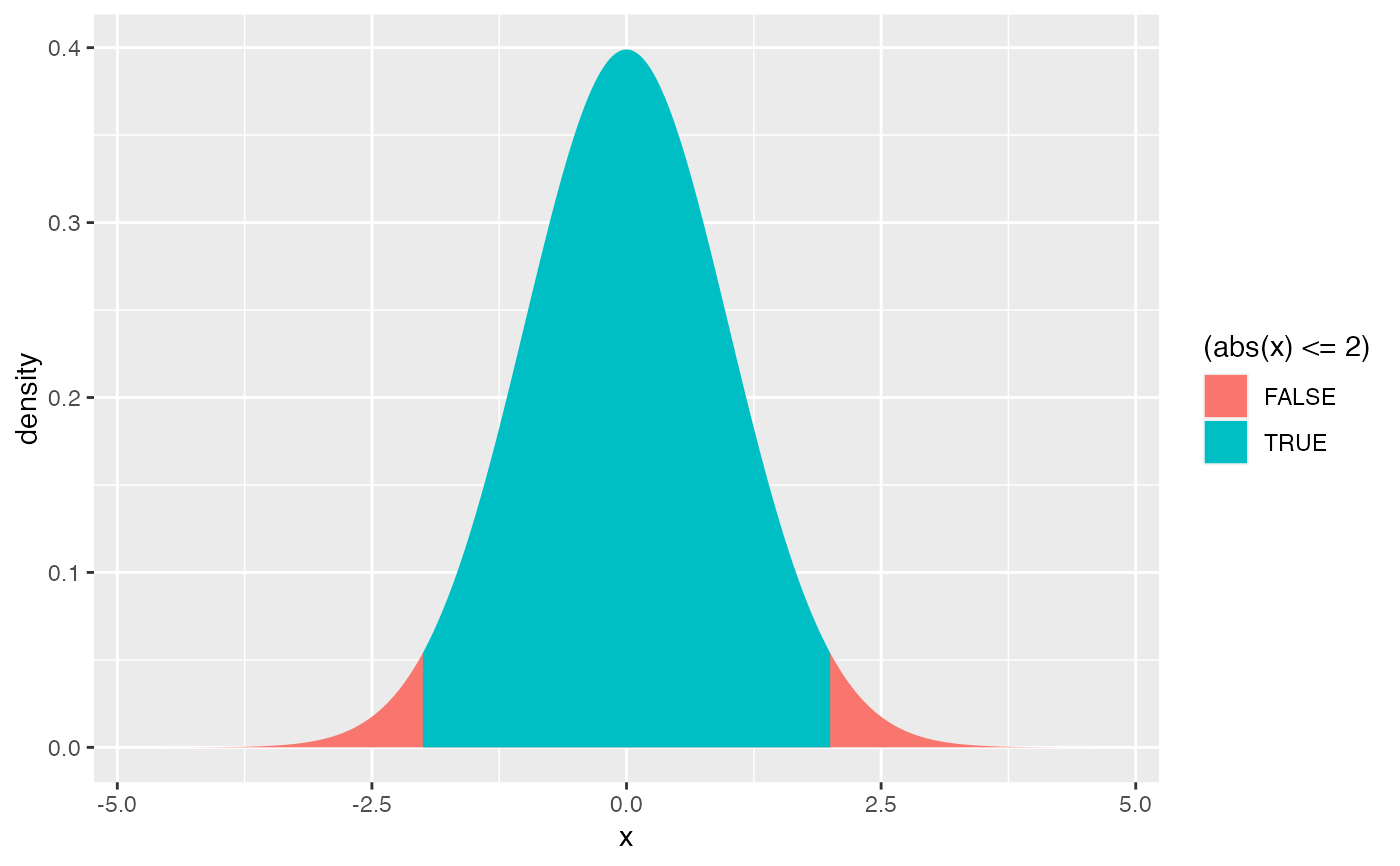
# shading tails -- but see pdist() for this
gf_dist("norm", fill = ~ (abs(x) <= 2), geom = "area")

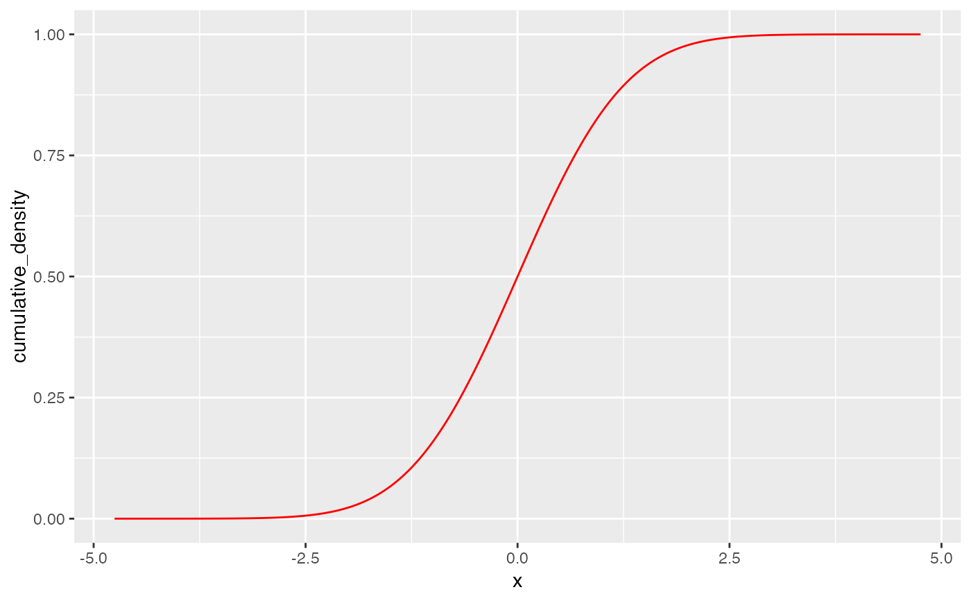
gf_dist("norm", color = "red", kind = "cdf")

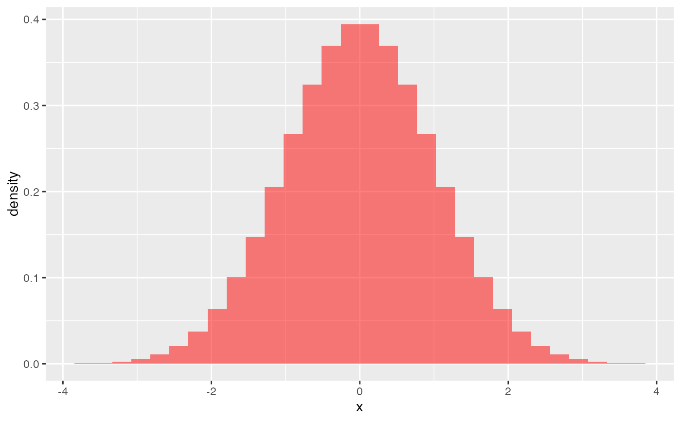
gf_dist("norm", fill = "red", kind = "histogram")
#> `stat_bin()` using `bins = 30`. Pick better value `binwidth`.

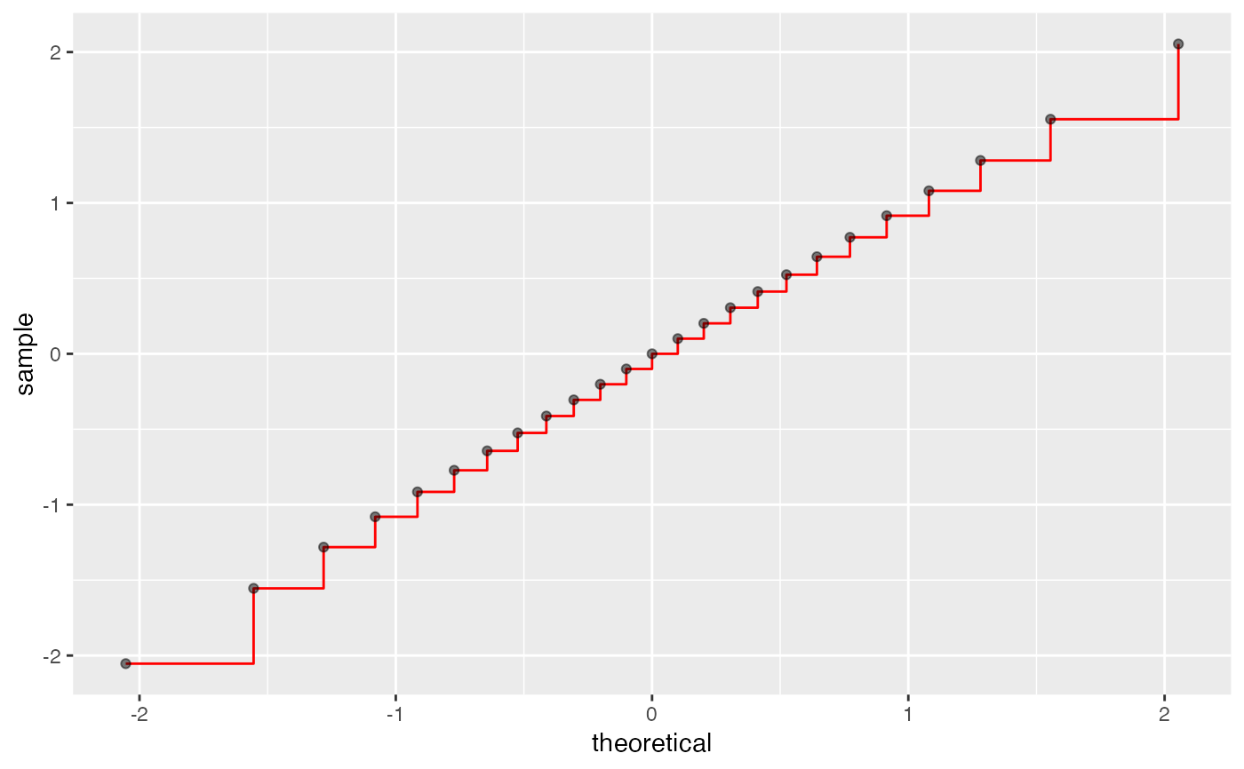
gf_dist("norm", color = "red", kind = "qqstep", resolution = 25) |>
  gf_dist("norm", color = "black", kind = "qq", resolution = 25, linewidth = 2, alpha = 0.5)

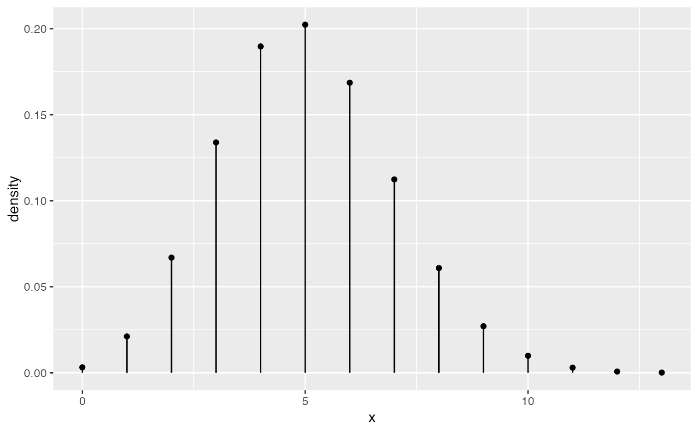
# size is used as parameter for binomial distribution
gf_dist("binom", size = 20, prob = 0.25)

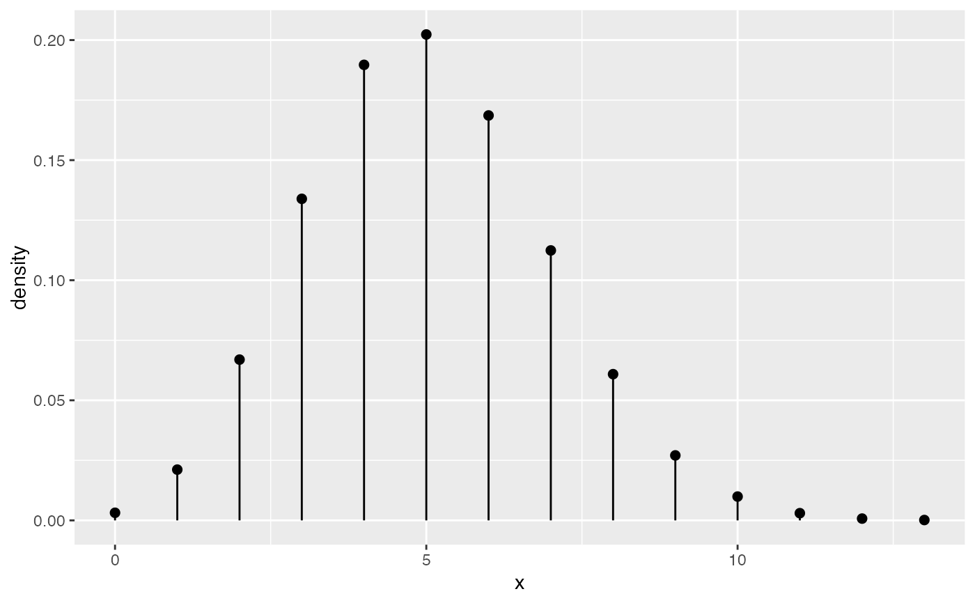
# If we want to adjust size argument for plots, we have two choices:
gf_dist("binom", size = 20, prob = 0.25, plot_size = 2)

gf_dist("binom", params = list(size = 20, prob = 0.25), size = 2)