Chapter 45 Statistical modeling and R2
So far, we’ve been looking at linear combinations from a distinctively mathematical point of view: vectors, collections of vectors (matrices), projection, angles and orthogonality. We’ve show a few applications of the techniques for working with linear combinations, but have always expressed those techniques using mathematical terminology. In this Chapter, we will take a detour to get a sense of the perspective and terminology of another field: statistics.
In the quantitative world, including fields such as biology and genetics, the social sciences, business decision making, etc. there are far more people working with linear combinations with a statistical eye than there are people working with the mathematical form of notation. Statistics is a far wider field than linear combination, so this chapter is not an attempt to replace the need to study statistics and data science. The purpose is merely to show you how a mathematical process can be used as part of a broader framework to provide useful information to decision-makers.
Since a statistics and data-science courses are part of a complete quantitative education, we want to point out from the beginning what you are likely to experience a traditional introductory statistics course and why that will seem largely disconnected from what you see here.
Statistics did not start out as a branch of mathematics, although people trained as mathematicians played a central role in it’s development. The story is complicated, but a simplification faithful to that history is to see statistics as an extension of biology. Statistics emerged in the last couple of decades of the 1800s. Possibly the key motivation was to understand genetics and Darwinian evolution. Today we know much about DNA sequences, RNA, amino acids, proteins, and so on. But quantitative genetics started in complete ignorance of any physical mechanism for genetics. Instead, mathematical models were the basis for the theory of genetics, beginning with with Gregor Mendel’s work on heritable traits published in 1865.1
Perhaps coincidentally—or perhaps not—Charles Darwin (1809-1882) was a half-cousin of Francis Galton (1822-1911). Traditional introductory statistics is based, more or less, on the work Galton and his contemporaries, for instance Karl Pearson (1857-1936) and William Sealy Gosset (1876-1937). The terms that you encounter in introductory statistics—correlation coefficient, regression, chi-squared test, t-test—where in place by 1910. Ronald Fisher (1890-1962), also a geneticist, extended this work based in part on the mathematical ideas of projection. Fisher invented analysis of variance (ANOVA) and maximum likelihood estimation and is perhaps the “great man” of statistics. (See Section 35.4 for an introduction to likelihood. We’ll briefly touch on ANOVA in this chapter.) To his historical discredit, Fisher was a leader in eugenics. He was also a major obstacle, to the statistical acceptance of the dangers of smoking.
Most of the many techniques covered in traditional introductory statistics are, in fact, manifestations of the application of a general technique: the target problem. They are not taught this way, partly out of hide-bound tradition and partly because the target problem has been covered, if at all, in the fourth or fifth semester of a traditional calculus sequence.
It often happens that a model is needed to help organize complex, multivariate data for purposes such as prediction. As a case in point, consider the data available in the Body_fat data frame, which consists of measurements of characteristics such as height, weight, chest circumference, and body fat on 252 men.
Znotes::and_so_on(Body_fat) %>% kableExtra::kable_minimal()| bodyfat | age | weight | height | neck | chest | abdomen | hip | thigh | knee | ankle | biceps | forearm | wrist |
|---|---|---|---|---|---|---|---|---|---|---|---|---|---|
| 12.3 | 23 | 154.25 | 67.75 | 36.2 | 93.1 | 85.2 | 94.5 | 59.0 | 37.3 | 21.9 | 32.0 | 27.4 | 17.1 |
| 6.1 | 22 | 173.25 | 72.25 | 38.5 | 93.6 | 83.0 | 98.7 | 58.7 | 37.3 | 23.4 | 30.5 | 28.9 | 18.2 |
| 25.3 | 22 | 154.00 | 66.25 | 34.0 | 95.8 | 87.9 | 99.2 | 59.6 | 38.9 | 24.0 | 28.8 | 25.2 | 16.6 |
| … and so on … | |||||||||||||
| 26.0 | 72 | 190.75 | 70.5 | 38.9 | 108.3 | 101.3 | 97.8 | 56.0 | 41.6 | 22.7 | 30.5 | 29.4 | 19.8 |
| 31.9 | 74 | 207.50 | 70.0 | 40.8 | 112.4 | 108.5 | 107.1 | 59.3 | 42.2 | 24.6 | 33.7 | 30.0 | 20.9 |
Body fat, the percentage of total body mass consisting of fat, is thought by some to be a good measure of general fitness. To what extent this theory is merely a reflection of general societal attitudes toward body shape is unknown.
Whatever its actual utility, body fat is hard to measure directly; it involves submerging a person in water to measure total body volume, then calculating the persons mass density and converting this to a reading of body-mass percentage. For those who would like to see body fat used more broadly as a measure of health and fitness, this elaborate procedure stands in the way. And so they seek easier ways to estimate body fat along the lines of the Body Mass Index (BMI), which is a simple arithmetic combination of easily measured height and weight. (Note that BMI is also controversial as anything other than a rough description of body shape. In particular, the label “overweight,” officially \(25 \leq \text{BMI}\leq 30\) has at best little connection to actual health.)
How can we construct a model, based on the available data, of body fat as a function of the easy-to-measure characteristics such as height and weight? You can anticipate that this will be a matter of applying what we know about the target problem \[\text{Given}\ \mathit{A}\ \text{and}\ \vec{b}\text{, solve } \mathit{A} \vec{x} = \vec{b}\ \text{for}\ \vec{x}\]where \(\vec{b}\) is the column of body-mass measurements and \(\mathit{A}\) is the matrix of all the other columns in the data frame.
In statistics, the target \(\vec{b}\) is called the response variable and \(\mathit{A}\) is the set of explanatory variables. You can also think of the response variable as the output of the model we will build and the explanatory variables as the inputs to that model.
Although application of the target problem is an essential part of constructing a statistical model, it is far from the only part. For instance, statisticians find is useful to think about “how much” of the response variable is explained by the explanatory variables. Measuring this requires a definition for “how much.” In defining “how much,” statisticians focus not on how much variation there is among the values in the response variable. The standard way to measure this is with the variance, which was introduce in Section 41.4 and can be thought of as the average of pair-wise differences among the elements in \(\vec{b}\).
In order to support this focus on the variance of \(\vec{b}\), statisticians typically augment \(\vec{A}\) with a column of ones, which they call the intercept.
To move forward, we’re going to extract the response variable from the data and construct \(\vec{A}\), adding in the vector of ones. We’ll show the vector/matrix commands for doing this, but you don’t have to remember them because statisticians have a more user-friendly interface to the calculations.
b <- with(Body_fat, cbind(bodyfat))
A <- Body_fat[-1] %>% as.matrix
A <- cbind(1, A)
x <- qr.solve(A, b)
The -1 in the second command is a directive to get rid of column 1, which happens to the the response variable, in constructing \(\vec{A}\).
Having applied qr.solve(), \(\vec{x}\) now contains the coefficients on the “best” linear combination of the columns in \(\vec{A}\). One of the ways in which the R language is designed to support statistics, is that it keeps track of names of columns, so the elements of \(\vec{x}\) are labelled with the name of the column the element applies to.
x## bodyfat
## -18.18848508
## age 0.06207865
## weight -0.08844468
## height -0.06959043
## neck -0.47060001
## chest -0.02386415
## abdomen 0.95477346
## hip -0.20754112
## thigh 0.23609984
## knee 0.01528121
## ankle 0.17399537
## biceps 0.18160242
## forearm 0.45202491
## wrist -1.62063910
Based on the above, the model for body fat as a function of the explanatory variables is:
\[\text{body fat} = -18.2 + 0.062\, \mathtt{age} - 0.0884\, \mathtt{weight} - 0.696\, \mathtt{height} + \text{an so on}\ .\]
Once we have the means to solve the target problem, as we do with qr.solve(), constructing such a model is straightforward.
But some questions remain: - How good is the model? - Could we make a better model?
To answer these questions, we’ll have to develop a measure of how good the model is. And this depends on the purpose for which we’ll be using the model.
45.1 R-squared
One of the most basic indices of the quality of a model—but far from the only one!—is a statistic written R2 and pronounced “R-squared.”
R2 is quite simple. Remember that a basic statistical question is how much variation there is in the response variable. That’s measured with the variance:
var(b)## bodyfat
## bodyfat 70.03582
We can also look at the variation in the model vector, \(\hat{b}\).
bhat <- A %*% x
var(bhat)
## bodyfat
## bodyfat 52.46033
R2 is simply the ratio of these two variances:
var(bhat) / var(b)## bodyfat
## bodyfat 0.74905
This result, 74.9%, is interpreted as the fraction of the variance in the response variable that is accounted for by the model. Near synonyms for “accounted for” is explained by or can be attributed to.
In the same spirit, we can ask how much of the variance in the response variable is unexplained by, or unaccounted by the explanatory variables. To answer this, look at the size of the residual:
var(b - bhat) / var(b)## bodyfat
## bodyfat 0.25095
Notice that the amount of variance explained, 74.905%, plus the amount remaining unexplained, 25.095%, add up to 100%. This is no accident. It is the reason why statisticians use the variance as a measure of variability.
Let’s re-do the calculations, but using the software interface designed for statistical modeling rather than the interface used for constructing matrices. In R, the core program is called lm(), which stands for “linear model.” The lm() interface combines the construction phase and the model fitting phase and is connected with other software for doing an analysis of the model.
mod_big <- lm(bodyfat ~ ., data = Body_fat)
coef(mod_big)
## (Intercept) age weight height neck chest
## -18.18848508 0.06207865 -0.08844468 -0.06959043 -0.47060001 -0.02386415
## abdomen hip thigh knee ankle biceps
## 0.95477346 -0.20754112 0.23609984 0.01528121 0.17399537 0.18160242
## forearm wrist
## 0.45202491 -1.62063910
rsquared(mod_big)## [1] 0.74905
The first argument to lm() is a tilde expression specifying the response variable (on the left of ~) and the explanatory variables. The vector of ones is included by default without needing to specify it. And there are some other shortcuts. For instance, in the tilde expression bodyfat ~ . the dot on the right-hand side of the tilde means “all the columns except the response variable.”
The results from lm() are, as you can see, identical to those produced by the matrix manipulations in the previous section.
45.2 Interpreting the model
One of the ways statistics differs from mathematics is that statistics is concerned with the interpretation of the model, the ways the model is or is not fit for purpose, and the ways the model can be improved.
Since the purpose of the body-fat model is to estimate the actual body fat percentage from easy-to-measure variables, let’s examine how much knowing the output of the model tells us about the actual body fat. We’ve already seen that R2 is 75%, but there are other ways to look at things. Figure 45.1 shows the actual body fat in each of the 252 men whose data are in Body_fat as a function of the model output.
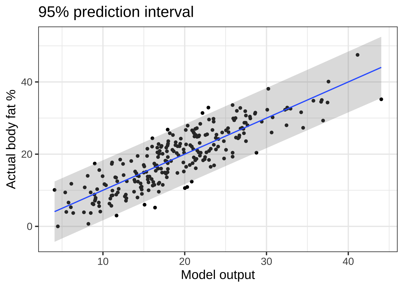
Figure 45.1: Comparing the output of the model to the actual body-fat measurements made in the 252 men represented in the Body_fat data frame.
Using the graph, consider what to make of a model output of 20. Looking at the dozen or so men whose measurements led to an output near 20, their actual body fat spans a range of values, from about 10% to 30%. The prediction error for any given man is the difference between the actual value of body fat and the model output. The gray band on the graph contains about 95% of all the men. The vertical width of the band—about -8% to +8%—gives a prediction error that encompasses 95% of the men. This is interpreted to mean that the model output reflects the actual body mass, plus-or-minus 8%. (There’s no guarantee that the prediction error will be \(\leq 8\%\), but in the large majority of cases (roughly 95%) the model output will have a prediction error that’s no larger than \(\pm 8\%\).)
Another difference between statistics and mathematics is that good statistical work always requires some understanding of the system being studied, not just the manipulation of columns of numbers. Look back at the coefficients. Some make sense and some are questionable. For instance, the positive coefficient on abdomen makes intuitive sense since everyday experience is that body fat often appears there. But the negative coefficient on neck, what’s that about?
45.3 Improving the model
The model that we built of body fat, which we called big_mod, might just as well have been called “kitchen sink.” It includes all possible explanatory variables. But it doesn’t have terms higher than first order. That is, neck enters into the model just as a linear function. But in Chapter 25 we introduced low-order polynomial terms, such as the quadratic neck^2 or the interaction neck*abdomen. Maybe we would do better by introducing such terms. Since there are 13 explanatory variables, this would add 13 quadratic terms and many interaction terms, one for each pair of variables. That’s 78 vectors for the interaction plus 13 linear terms plus another 13 quadratic terms.
Let’s try adding these interaction terms a few at a time to see what happens. The modeling syntax for interaction terms uses the multiplication symbol *. We’ll compare the new models to big_mod which had an R2 of 74.9%.
mod2 <- lm(bodyfat ~ . * neck, data = Body_fat)
rsquared(mod2)
## [1] 0.7730899
Including the interactions with neck has increased R2 to 77.3%. Let’s keep going:
mod3 <- lm(bodyfat ~ . * neck + . * weight + . * abdomen, data=Body_fat)
rsquared(mod3)
## [1] 0.7932603
Again, R2 has gone up! Unfortunately, adding more terms is not a sure-fire way to improve a model. In model 3, we added 12 vectors from *.neck, 11 from .*weight, 10 from .*abdomen. (The reason for the decreasing counts is that .*neck already includes weight*neck, so the neck*weight that’s included in . * weight is redundant.) Adding altogether 33 new vectors on top of the 13 in the original model, has increased the R2 from 74.9% to 79.3%. That’s a gain of 4.4 percentage points from 33 new vectors.
Is that gain worth it? To answer that question, we need to consider what is the cost induced by adding the 33 new vectors. The computational cost is not the issue, since even much bigger models are easily constructed on ordinary laptops. The issue has to do with the goal of predicting bodyfat. We don’t need to predict body fat for the men in the data; we already know their body fat. Instead, the point is to make predictions for men not in the data. These two kinds of prediction are called in-sample prediction (men in the data set) and out-of-sample prediction (men not in the data set).
The problem is that in-sample predictions tend to have a larger R2 than out-of-sample predictions. And it’s the out-of-sample prediction that will matter in applications: predictions for people whose body fat is unknown and therefore will be estimated from the model.
A major goal in statistics and machine learning is to estimate the R2 for out-of-sample prediction from just the data in the sample itself. Here’s one way to get at the out-of-sample prediction error: divide the data at random into two halves, fitting the model on the first half and estimating the out-of-sample prediction error using the other half, the half that is out-of-sample for fitting the model. This strategy, and many refinements to it, are called cross-validation and is a major technique in machine learning.
An older statistical technique gets at the problem of in- and out-of-sample by using models constructed from random stand-ins for explanatory vectors. For instance, we can examine whether the 33 interaction terms we added to the model are contributing to prediction by replacing them with 33 random vectors and examining the gain in R2 from that. Here’s one way to do this, using rand(33) to generate the random variables:
mod3R <- lm(bodyfat ~ . + rand(33), data=Body_fat)
rsquared(mod3)
## [1] 0.7932603
The random variables did every bit as well as the interaction terms! So there’s no particular reason to think that the interaction terms are contributing to the prediction.
The example we just gave with . + rand(33) isn’t completely adequate to the statistician’s needs. Those 33 random vectors were just a particular random choice, a role of the vector dice. We need to establish whether the result we got, R2=79.3% was just good luck. The next code block shows one way to do this: we generate many trials of rand(33), calculating R2 for each trial. Then compare the “genuine vectors” result to the distribution of results from the random trials.
You do not need to learn how to construct such code, but perhaps you will be able to gain some insight from it. We’re doing 100 random trials.
trials <- do(100) * {lm(bodyfat ~ . + rand(33), data=Body_fat) %>% rsquared()}
table(rsquared(mod3) > trials)
##
## FALSE TRUE
## 14 86
The “genuine vectors” gave a result bigger than 90 out of 100 trials. This sort of “most of the time” doesn’t cut muster. A convention is to insist that the genuine vectors win at least 95% of the time. The 90-out-of-100 result would typically be reported as a p-value less than 10%.
Another sort of standard statistical report carries out this same sort of comparison to random vectors, but building up the model one term at a time. This is called analysis of variance. A standard report looks like this:
anova(mod_big)## Analysis of Variance Table
##
## Response: bodyfat
## Df Sum Sq Mean Sq F value Pr(>F)
## age 1 1493.3 1493.3 80.5644 < 2.2e-16 ***
## weight 1 6674.3 6674.3 360.0837 < 2.2e-16 ***
## height 1 1043.0 1043.0 56.2712 1.250e-12 ***
## neck 1 152.4 152.4 8.2227 0.004508 **
## chest 1 641.1 641.1 34.5856 1.373e-08 ***
## abdomen 1 2757.4 2757.4 148.7645 < 2.2e-16 ***
## hip 1 22.5 22.5 1.2157 0.271327
## thigh 1 110.6 110.6 5.9665 0.015309 *
## knee 1 0.0 0.0 0.0013 0.971409
## ankle 1 0.1 0.1 0.0043 0.948064
## biceps 1 45.2 45.2 2.4369 0.119842
## forearm 1 57.5 57.5 3.1013 0.079514 .
## wrist 1 170.1 170.1 9.1781 0.002720 **
## Residuals 238 4411.4 18.5
## ---
## Signif. codes: 0 '***' 0.001 '**' 0.01 '*' 0.05 '.' 0.1 ' ' 1
The first row of the report examines how well the model with just age does compared to random vectors. As you can see, the p-value (column Pr(>F)) is much smaller than the standard cut-off of 0.05. The next row in the report gives the improvement in the model when weight is included along with age in the model. And so on down the line.
The report highlights some stinkers among the explanatory variables: hip, knee, ankle, and biceps. Maybe this matches your intuition, for instance that ankle circumference is not the best way to look at body fat.
This sort of analysis, which has many nuances not covered here, falls under the name statistical inference. Another, more recent term is statistical learning, often called machine learning. The general idea of statistical or machine learning is to search through many combinations of possible explanatory variables to construct a “best” model. This search often involves models that are not simply linear combinations. Some of these model architectures have catchy names: “deep learning,” “neural nets,” “support vector machines,” “lasso,” and so on. Very often, these machine learning models are built by gradient descent, and are elaborations of the basic \(\mathit{A}\vec{x} = \vec{b}\) model architecture. But they often have capabilities beyond \(\mathit{A}\vec{x} = \vec{b}\). For instance, deep learning and lasso are designed to handle situations where the number of explanatory variables—the number of columns in the data frame—is far larger than the number of rows. An example: learning to identify whether there is an animal in a photograph with 20,000 pixels. And returning to genetics: measuring 100,000 genetic expression products on a sample of 10 people with a disease and 10 healthy controls to determine which, if any, genes are related to the disease.
45.4 Machine learning
If you pay attention to trends, you will know about advances in artificial intelligence and the many claims—some hype, some not—about how it will change everything from animal husbandry to warfare. Services such as Google Translate are based on artificial intelligence, as are many surveillance technologies. (Whether the surveillance is for good or ill is a serious matter.)
Skills in artificial intelligence are currently a ticket to lucrative employment.
Like so many things, “artificial intelligence” is a branding term. In fact, what all the excitement is about is not mostly artificial intelligence at all. The advances, by and large, have come over 50 years of development in a field called “statistical learning” or “machine learning,” depending on whether the perspective is from statistics or computer science.
A major part of the mathematical foundation of statistical (or “machine”) learning is linear algebra. Many workers in “artificial intelligence” are struggling to catch up because they never took linear algebra in college or, if they did, they took a proof-oriented course that didn’t cover the elements of linear algebra that are directly applicable. We’re trying to do better in this course.
So if you’re diligent, and continue your studies to take actual statistical/machine learning courses, you’ll find yourself at the top of the heap. Even xkcd, the beloved techno-comic, gets in on the act, as this cartoon reveals:
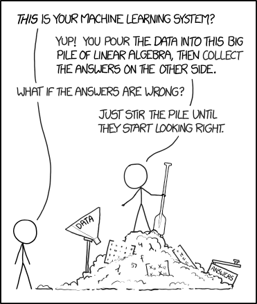 Look carefully below the paddle and you’ll see the Greek letter “lambda”, \(\lambda\). You’ll meet the linear algebra concept signified by \(\lambda\)—eigenvalues and eigenvectors—in Block 6.
45.5 Exercises
Exercise XX.XX:  97zwR6
A. What’s the largest possible value for R2?
As you know, R2 is a ratio of variances. A good way to think of variance is as the square length of a vector. So think about R2 as if it were calculated from the square length of \(\vec{b}\) and \(\hat{b}\).
(Hint: What does the projection problem tell you about the lengths of \(\vec{b}\) and \(\hat{b}\).)
B. What’s the smallest possible value for R2? (Hint: What’s the smallest possible length for \(\hat{b}\)?)Exercises confirming that qr.solve() produces results that are as they should be: residual orthogonal to every vector in A, projected + residual = \(\vec{b}\).
Exercises confirming that adding more columns to A produces a smaller residual.
Demonstration that even random vectors can be combined to exactly equal \(\vec{b}\), so long as we have enough of them.
Amazingly, this work attracted little attention until after 1900, when Mendel’s laws were rediscovered by the botanists de Vries, Correns, and von Tschermak.↩︎