Chapter 36 Present and future value
Comparison is an important element of human decision making. Often, comparison amounts to translating each of the options at hand into a scalar score. (Recall that a scalar is just an ordinary quantity, e.g. 73 inches. As we get more deeply involved with vectors it will become more important to be perfectly clear when we are talking about a vector and when about a scalar. So we’ll be using “scalar” a lot.) Scalars are easy to compare; the skill is taught in elementary school. Scalar comparison is completely objective. Putting aside the possibility of error, everyone will agree on which of two numbers is bigger. Importantly, comparison of scalars is transitive, that is if \(a > b\) and \(b > c\) then it is impossible that \(a \leq c\).
The comparison of scalars can be extended to situations where the options available form a continuum and the score for each option \(x\) is represented by a function, \(f(x)\). As we saw in Chapters 23 and 34 selecting the highest scoring option is a matter of finding the argmax.
Many decisions involve options that have two or more attributes that are not directly comparable. Expenditure decisions have this flavor: Is it worth the money to buy a more reliable or prettier or more capable version of a product? The techniques of constrained optimization (Chapter 34) provide one useful approach for informing decisions when there are multiple objectives.
Elections are a form of collective decision making. The options—called, of course, “candidates”—have many attributes. Three such attitudes are attitudes toward social policy, toward fiscal policy, and toward foreign policy. Perceived honesty and trustworthiness as well as the ability to influence other decision makers and perceived ability to win the election are other attributes that are considered and balanced against one another. Ultimately the decision is made by condensing the diverse attributes into a single choice for each voter. The election is decided by how many votes the candidate garners. With this number attached to each of the candidates, it’s easy to make the decision, \[\text{winner} \equiv\mathop{\text{argmax}}_{i} \text{votes}(\text{candidate}_i)\ .\] There are many voting systems. For instance, sometimes the winner is required to have a majority of votes and, if this is not accomplished, the two highest vote-getting candidates have a run-off. Some jurisdictions have introduced “rank-choice” voting, where each voter can specify a first choice, a second choice, and so on. US federal elections involve a primary system where candidates compete in sub-groups before the groups complete against one another. It’s tempting to think that there is a best voting system if only we were clever enough to find one and convince authorities to adopt it. But two mathematical theorems, Arrow’s impossibility theorem and the Gibbard-Satterthwaite theorem demonstrate that this is not the case for any system that involves three or more candidates. All such voting systems potentially create situations where a voter’s sincere interests are best served by an insincere, tactical vote choice. A corollary is that voters can be tricked into making a sincere choice that violates their interests.
This chapter is about a very common situation where there are multiple attributes that need to be condensed into a single score. The setting is simple: money. The question is how to condense a future income/expense stream—a function of time—into an equivalent value of money in hand at the present. This is called the present value problem. There is a solution to the problem that is widely accepted as valid, just as voting is a hallowed process of social optimization. But like voting, with its multiplicity of possible forms, there is a subtlety that renders the result somewhat arbitrary. This is not a situation where there is a single, mathematically correct answer but rather a mathematical framework for coming to sensible conclusions.
Consider the situation faced by an entrepreneur who is considering constructing an 8-rental-unit apartment building. The planning and construction process takes time and money. Let’s assume that $3,000,000 will be spent over three years to locate a suitable property, get the needed licenses and approvals, and build. For simplicity, we’ll model that by a piecewise function \(\text{construction}(t)\): \[\text{construction}(t) \equiv \left\{\begin{array}{c} 1,000,000\ \text{per year} & \text{for}\ 0 \leq t \leq 3\\0& \text{thereafter.} \end{array} \right.\] Suppose the planned rent will be $3000 per month per apartment. That suggests $36,000 in rental income per apartment each year, but typically there are vacancies or renters who fail to pay, so let’s assume $32,000 per unit per year. For the 8-apartments, that’s a total rental income of $250,000 per year: \[\text{rental}(t) \equiv \left\{\begin{array}{c} 0 & \text{for}\ 0 \leq t \leq 3\\250,000\ \text{per year}& \text{thereafter.} \end{array} \right.\] Maintenance is an additional expense. We’ll put that as a increasing function of \(t\), starting at $50,000 per year when the building is complete (at the end of year 3) and rising linearly to $200,000 per year at the end of the 30-year project: \[\text{maintenance}(t) \equiv \left\{\begin{array}{c} 0 & \text{for}\ 0 \leq t \leq 3\\33333 + 5556 t\ \ \text{per year}& \text{thereafter.} \end{array} \right.\]
Finally, assume that the business plan is to sell the building in year 30, at which point it is assumed to be worth $1,000,000:
\[\text{sale}(t) \equiv \left\{\begin{array}{c} 1,000,000\ \text{per year} & \text{for}\ 29 < t < 30\\0 & \text{otherwise}\end{array}\right.\] The income stream stops for \(30 < t\).
Altogether, the income stream is \[\text{income}(t) = \text{sale}(t) + \text{rental}(t) - \text{construction}(t) - \text{maintenance}(t)\ .\] Notice that construction and maintenance are considered as negative income. Figure 36.1 shows a graph of \(\text{income}(t)\).
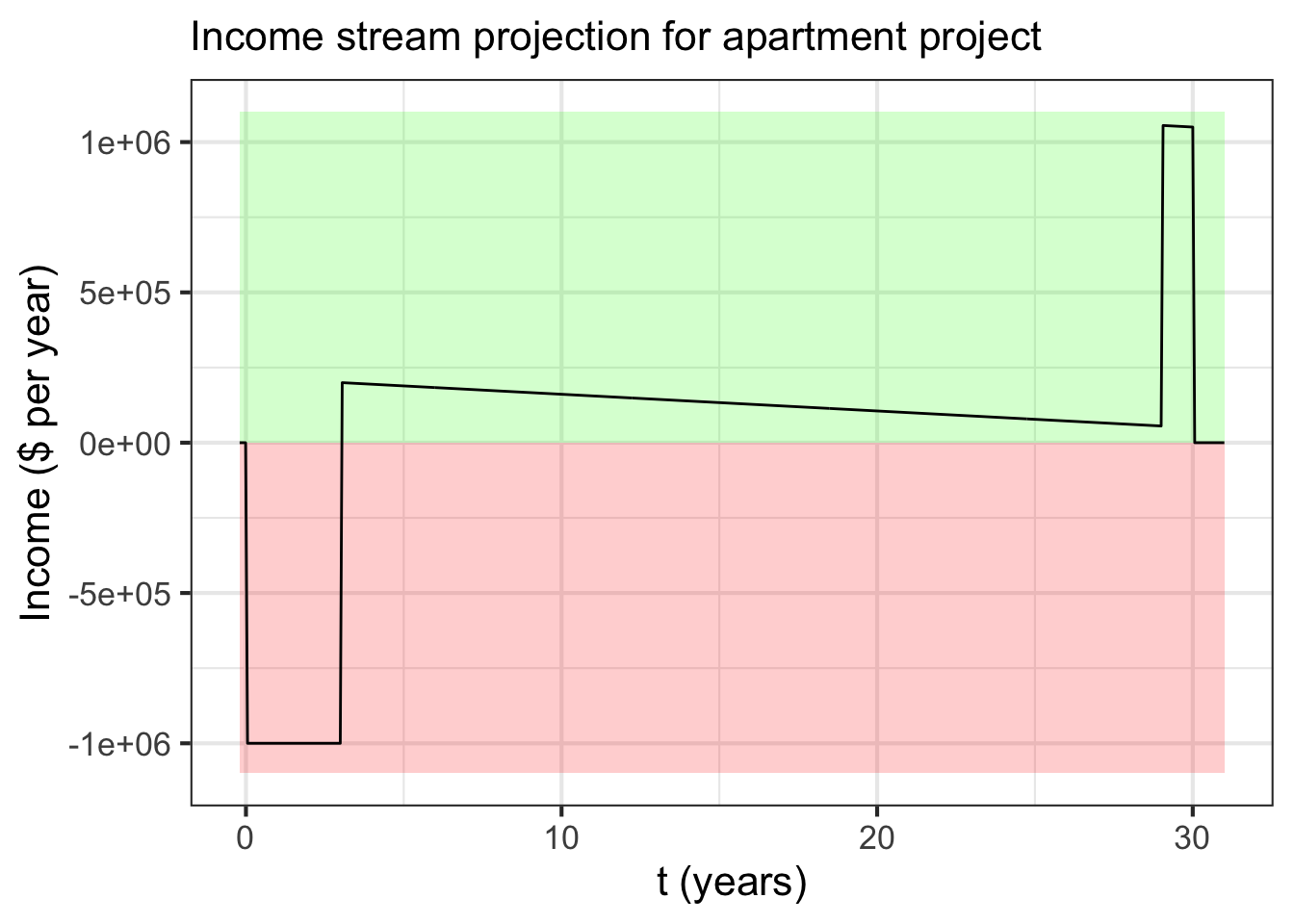
Figure 36.1: The income stream for an apartment-building project. Following convention, positive income is “in the green”, and negative income is “in the red”.
36.1 Present value
People and institutions often have to make decisions about undertakings where the costs and benefits are spread out over time. For instance, a person acquiring an automobile or home is confronted with a large initial outlay. The outlay can be financed by agreeing to pay amounts in the future, often over a span of many years.
Another example: Students today are acutely aware of climate change and the importance of taking preventive or mitigating actions such as discouraging fossil fuel production, investing in renewable sources of energy and the infrastructure for using them effectively, and exploring active measures such as carbon sequestration. The costs and benefits of such actions are spread out over decades, with the costs coming sooner than the benefits. Policy makers are often and perhaps correctly criticized for overvaluing present-day costs and undervaluing benefits that accrue mainly to successive generations. There are many analogous situations on a smaller scale, such as setting Social Security taxes and benefits or the problem of underfunded pension systems and the liability for pension payments deferred to future taxpayers.
The conventional mechanism for condensing an extended time stream of benefits and costs is called discounting. Discounting is based on the logic of financing expenditures via borrowing at interest. For example, credit cards are a familiar mechanism for financing purchases by delaying the payment of money until the future. An expense that is too large to bear is “carried” on a credit card so that it can be paid off as funds become available in the future. This incurs costs due to interest on the credit-card balance. Typical credit-card interest rates are 18-30% per year.
As notation, consider a time stream of income \({\cal M}(t)\), as with the apartment building example. We’ll call \({\cal M}(t)\) the nominal income stream with the idea that the money in \({\cal M}(t)\) is to be counted at face value. “Face value” is the literal amount of the money. In the case of cash, a $20 bill has a face value of $20 regardless of whether it becomes available today or in 50 years. The word “nominal” refers to the “name” on the bill, for instance $20.
The big conceptual leap is to understand that the present value of income in a future time is less than the same amount of income at the present time. In other words, we discount future money compared to present money. For example, if we decide that an amount of money that becomes available 10 years into the future is worth only half as much as that same amount of money if it were available today, we would be implying a discounting to 50%. In comparison, if that money were available 20 years in the future, it would make sense to discount it by more strongly to, say, 25%.
To represent the discounting to present value as it might vary with the future time horizon, we multiply the nominal income stream \({\cal M}(t)\) by a discounting function \({\cal D} (t)\). The function \({\cal D}(t)\, {\cal M}(t)\) gives the income stream as a present value rather than a nominal value. It’s sensible to insist that \({\cal D} (t=0) \equiv 1\) which is merely to say that the present value of money available today is exactly the same as the nominal value.
The net present value (NPV) of a nominal income stream \({\cal M}(t)\) is simply the sum of the stream discounted to the present value. Since we’re imagining that the income stream is a function of continuous time, the sum amounts to an integral: \[\text{NPV} \int_\text{now}^\text{forever} {\cal M}(t)\ {\cal D}(t)\, dt\ .\]
36.2 Discounting functions
What should be the shape of the discounting function?
Recall that the purpose of the discounting function is to help us make comparisons between different income streams, that is, between the various options available to an entrepreneur. Each individual can in principle have his or her own, personal discounting function, much as each voter is entirely free to weight the different attributes of the candidates when deciding whom to vote for. As a silly example, a person might decide that money that comes in on a Tuesday is lucky and therefore worth more than Thursday money. We won’t consider such personalized forms further and instead emphasize discounting functions that reflect more standard principles of finance and economics.
As a thought experiment, consider the net present value of an income stream, that is \[\text{NPV}_\text{original} = \int_0^\infty {\cal M}(t)\ {\cal D}(t)\, dt\ .\] Imagine now that it has been proposed to delay the income stream by \(T=10\) years. This new, delayed income stream is \({\cal M}(t-T)\) and also has a net present value: \[\text{NPV}_\text{delayed} = \int_0^\infty {\cal M}(t - T)\ {\cal D}(t)\, dt\ .\] There are at least two other ways to compute \(\text{NPV}_\text{delayed}\) that many people would find intuitively reasonable:
- Simply discount the original NPV to account for it becoming available \(T\) years in the future, that is, \[\text{NPV}_\text{delayed} = {\cal D}(T)\ \text{NPV}_\text{original} = \int_0^\infty {\cal M}(t)\ {\cal D}(T)\ {\cal D}(t)\, dt\ \]
- Apply to \({\cal M}(t)\) a discount that takes into account the \(T\)-year delay. That is:
\[\text{NPV}_\text{delayed} = \int_0^\infty {\cal M}(t)\ {\cal D}(t + T)\, dt\ .\] For (1) and (2) to be the same, we need to restrict the form of \({\cal D}_r(t)\) so that \[{\cal D}(T)\ {\cal D}(t) = {\cal D} (t+T)\ .\] The form of function that satisfies this restriction is the exponential, that is \({\cal D}(t) \equiv e^{kt}\).
36.3 Compound interest
A more down-to-earth derivation of the form of \({\cal D}(t)\) is to look at how financial transactions take place in the everyday world: borrowing at interest. Suppose that a bank proposes to lend you money at an interest rate of \(r\) per year. To receive from the bank one dollar now entails that you pay the bank \(1+r\) dollars at the end of the year.
For this proposition to be attractive to you, the present value of \(1+r\) dollars to be paid in one year must be less than or equal to the present value of one dollar today. In other words, \[{\cal D}_\text{you}(1)\ (1+r) \leq 1\ .\] From the bank’s perspective, the present value of your payment of \((1+r)\) dollars in a year’s time must be greater than one dollar today. That is
\[1 \leq {\cal D}_\text{bank}(1)\ (1+r) \ .\] It’s perfectly reasonable for you and the bank to have different discounting functions, just as it’s perfectly legitimate for you and another voter to have different opinions about the candidates. It’s convenient, though to imagine that the two discounting functions are the same, which will be the case if \[{\cal D}(1) = \frac{1}{1+r}\ .\]
If you were to borrow money for two years, the bank would presumably want to charge more for the loan. A typical practice is to charge compound interest. Compound interest corresponds to treating the loan as having two phases: first, borrow one dollar for a year and owe \(1+r\) dollars at the end of that year. At that point, you will borrow \((1+r)\) dollars at the interest rate \(r\). At the end of year two you will owe \((1+r) (1+r) = (1+r)^2\) dollars. In general, if you were to borrow one dollar for \(t\) years you would owe \((1+r)^t\) dollars. In order for the loan to be attractive to both you and the bank, the discounted value of \((1+r)^t\) should be one dollar: \[{\cal D}(t) = \frac{1}{(1+r)^t} = (1 + r)^{-t}\ .\]
Let’s return to the entrepreneur considering the apartment-building project.
The entrepreneur goes to the bank with her business plan and financial forecasts. The bank proposes to lend money for the project at an interest rate of 7% per year.
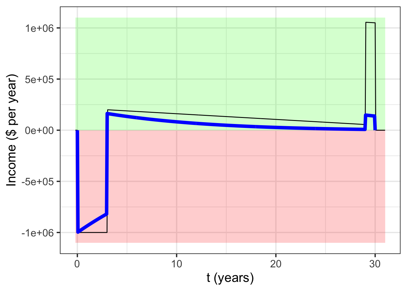
Figure 36.2: Blue curve: The apartment project income stream discounted at 7% per year. Black curve: The undiscounted income stream.
Figure 36.2 shows the income stream discounted at 7% per year. The net present value of the income stream for the apartment project is the accumulation of the discounted income stream: \[\text{NPV}(7\%) = \int_0^{30} (1 + 0.07)^{-t} {\cal M}(t) \ dt \ .\] This works out to be negative $1,095,000. As things stand, the apartment building will be a money pit.
The entrepreneur responds to the bank’s offer with some business jargon. “I’ll have to go back to the drawing board, put the team’s heads together, and see how to get the numbers to work. I’ll circle back with you tomorrow.” This might involve reconsidering her model of the income stream. Perhaps she should have taken into account yearly rent increases. Maybe she can re-negotiate with the city about zoning height restrictions and build a 12-unit building, which will cost $4 million, lowering the cost per apartment?
36.4 Mortgages
A mortgage is a form of loan where you pay back the borrowed amount at a steady rate, month by month. At the end of a specified period, called the term of the mortgage, your have completely discharged the debt.
Suppose you decide to buy a product that costs \(\$\cal P\), say \(\cal P=\) $10,000 for a used car. Let’s say you need the car for your new job, but you don’t have the money. So you borrow it.
Your plan is to pay an amount \(A\) each month for 30 months—the next \(2\,\small\frac{1}{2}\) years. What should that rate be?
You can put the purchase on your credit card at an interest rate of \(r=2\%\) per month. This corresponds to \(k = \ln(1+r) = 0.0198\) per month. The net present value of your payments over 30 months at a rate of \(A\) per month will be
\[\int_0^{30} A {\cal D}_r(t)\, dt = \int_0^{30} e^{-kt} A = -\frac{A}{k} e^{-kt}\left.{\Large\strut}\right|_{t=0}^{30}\\ =- A \left(\strut \frac{e^{-30k}}{k} - \frac{e^{-0k}}{k} \right)\\ = - A\left(\strut27.88 - 50.50\right) = 22.62 A\]
The loan will be in balance if the net present value of the payments is exactly the same as the amount \({\cal P}\) you borrowed. For this 30-month loan, this amounts to \[22.62 A = {\cal P}\ ,\] from which you can calculate your monthly payment \({\cal A}\). For the $10,000 car loan, your monthly payment will be $10,000/22.62 or $442.09.
36.5 Exercises
Exercise 36.02:  YMoHRB
Verify that the restriction \[{\cal D}(T)\ {\cal D}(t) = {\cal D} (t+T)\] is satisfied, for any \(T\) when \[{\cal D}(t) \equiv e^{k t}\ .\]
Also, confirm that, with this definition for \({\cal D}(t)\), we have
\[{\cal D}(t=0) = 1\ .\]
Exercise 36.04: Dg7Qxv
The mathematician’s preferred format for discounting functions is \(e^{kt}\), while the banker’s is \((1+r)^{-t}\).
Derive an expression for \(k\) in terms of \(r\) so that the mathematician’s and banker’s forms are completely equivalent.
Use the computer to confirm your expression by plotting out both \((1+r)^{-t}\) and \(e^{kt}\), with \(k\) set according to your expression. (Hint: Pick a particular interest rate, say \(r=7\%\).)
Exercise 36.06: paP4qf
The Powerball is a weekly lottery famous for its outsized payoff. For instance, for the week of April 7, 2021, the jackpot payout was officially described as $43,000,000. But they don’t really mean this.
After withholding taxes, the supposed $43,000,000 amounts to $17,161,778 as a one time cash payment, or, alternatively, 30 annual payments of $873,711. (The tax numbers are for Colorado.) We want to find the discount rate that is implicit in the equating of $17M now with 30 payments of $875,000.
Discounted at a continuously compounded rate of \(k\), the net present value of a 30-year payment stream of $875K per year is \[\text{NPV}(k) = \int_0^{30} e^{-kt}\ \$875000\, dt\ .\]
- Solve this definite integral symbolically to find a formula for NPV\((k)\).
Using a sandbox, implement the function NPV\((k)\) in R.
Solve for \(k_0\) that gives NPV\((k_0) = \$17,000,000\).
Translate the continuously compounded interest rate \(k\) into the corresponding 1-year compounded interest rate \(r\).
There is a joke that makes sense only to the financially savvy: When the Powerball claims a $1 million payout, they mean $1 per year over a million years. We can do this calculation using the symbolic formula for NPV(t) but replacing the $875,000 with $1 and the 30 years upper limit of the integral with 1,000,000 years.
- Set the discount rate to the \(k_0\) you found in step (3) and calculate the net present value of $1 per year for a million years.
Exercise 36.08: tm0XB4
In this exercise, you’ll calculate the net present value of the social security payments for a woman retiring at age 70. We’ll assume that benefits are paid at a rate of $24,000 per year.
The following R/mosaic commands will construct a function, survive(age) that gives the proportion of people alive at age 70 who will survive to an older age. (This is estimated from the Social Security mortality tables for 2014.)
survive <- M2014F %>%
  filter(age >= 70) %>%
  select(age, nliving) %>%
  mutate(survival = nliving / 82818) %>%
  spliner(survival ~ age, data = .)
For a person living to age 100, the net present value at age 70 of the $24,000 annual social security benefit is \[\int_{70}^{100} 24000 \exp(-k*(age-70))\, dt\] Calculate this amount for a continuously compounded interest rate of \(k=0.03\) per year
- Benefit payments stop when a beneficiary dies. Of course, it’s not known ahead of time when a retiree will die, but the
survive(age)function gives a probability of surviving to any given age.
Modify the integral to incorporate the survival probability into the net present value calculation. That is, calculate the expectation value of the net present value.
- Is
survive(age)a probability density function? Explain why or why not.
Exercise 36.10: qgt0RV
Under Construction
Content subject to revision.
We have records of large earthquakes going back 1000’s of years, at least in those parts of the world that kept written records. In regions with mainly oral traditions, stories of historical earthquakes are treated with skepticism.
For instance, in California written records reach about 400 years into the past. Anticipating a future earthquakes is an everyday matter in California and governments in seismically active zones have prepared by means of building codes and emergency precautions. A bit further up the US West Coast, in the Cascadia region of Oregon, there is a shorter written record and, until the last 30-40 years, little realization that the area has been subject to profoundly powerful earthquakes called “great quakes.” There are great quakes in living memory: the 2004 Boxing Day earthquake centered on Sumatra that led to the deaths of hundreds of thousands of people, and the 2011 Tohoku earthquake in Japan that killed tens of thousands and led to the meltdown of nuclear power plants in Fukashima. Both of these were magnitude 9.1. Even larger were the 1964 9.2 magnitude quake in southern Alaska and the magnitude 9.5 Valdivia earthquake in Chile in 1960. The local magnitude scale is logarithmic, so a 9.5 magnitude quake releases about 3 times the energy of a 9.1 magnitude quake.
This exercise explores a model to inform the extent to which it’s worth preparing for such quakes in order to prevent material damage. The risk to life is another important matter. But feasible investments in the build environment can minimize the direct impact of earthquakes to human life. Tsunamis generated by quakes are another matter, for which the only effective mitigating precautions are the development of evacuation routes and procedures and relocation of building away from the affected zone.
Let’s imagine a situation in which $100 spent in precautions such as strengthening building construction would generate $1000 in savings in the event of a major earthquake. (This ratio is made up for demonstration purposes, but you can easily substitute a better substantiated estimate.) From a societal point of view, many people would see the investment as clearly worthwhile. But we’re going to take a more technical point of view that incorporates two factors:
- The $100 is to be spent today, while the $1000 savings will occur in the future. This can be handled by simple discounting.
- The time until the earthquake is unknown, although reasonable probability models are available.
The time of the last great Cascadia Zone earthquake is known with surprising precision: January 26, 1700. Before this, dates are estimated from geologic evidence. The figure shows the known history of Cascadia Zone earthquakes. Source
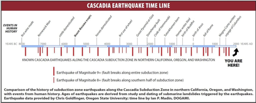
A standard model for the interval between earthquakes of a given magnitude is the exponential distribution. For the great quakes in the Cascadia Zone, the average interval between consecutive quakes is about 300 years and the corresponding exponential probability distribution is \[\frac{e^{t/300}}{300}\] The sandbox is set up to make a graph of this distribution and enables other calculations you will need later.
As shown by the definite integral already coded in the sandbox, the total probability of an earthquake at some point in the future is, according to the model, 100%. So this is a model of when an earthquake will occur, not whether one will occur.
prob <- makeFun(exp(-t/300)/300 ~ t)
slice_plot(prob(t) ~ t, domain(t = c(0,1000)))
Prob <- antiD(prob(t)~ t)
Prob(Inf) - Prob(0)
Almost everyone who meets the exponential probability model is surprised that the density is highest at time \(t=0^+\), that is, immediately after the previous quake.
Question A By using the appropriate definite integral, find the probability for earthquakes separated on average by 300 years (this essentially means using the provided model in the code) that the actual interval from the last quake will be less than 30 years. Which percentage is closest?
2%︎✘ 10%\(\heartsuit\ \) 20%︎✘ 25%︎✘
Question B Similarly to the previous question, find the probability that the actual interval from the last quake will be more than 500 years. (Hint: Be thoughful about what the limits of integration will be.)
2%︎✘ 10%︎✘ 20%\(\heartsuit\ \) 25%︎✘
An astounding and counter-intuitive aspect of the exponential model is that the same probability density describes the time from now to the eventual earthquake. In other words, it doesn’t matter how long it’s been since the last earthquake.
Now let’s put together our model of the net present value of an expenditure on earthquake preparedness. As you recall, the net present value of \(\$10\) to be paid \(t\) years from the present is \(10 e^{-r t}\), where \(r\) is the continuously compounded interest rate. For the example, we’ll set \(r=7.8\%\), as we did in the Powerball example.
Of course \(t\) is uncertain, so there’s no definite answer for the net present value of earthquake preparedness. However, since we have a model of the probability of the earthquake occuring as a function of the interval \(t\), we can find the expectation value of the net present value of earthquake preparedness.
For continuous probability densities (such as the exponential earthquake interval model) an expectation value is the definite integral over all possibilities of the probability density times the eventual outcome.
Question C Using the information presented above about the probability density function and the net present value, which of the following is appropriate for calculation of the net present value of $10 spent today for earthquake preparedness?
- \(\frac{100}{300} \int_{0}^{\infty} e^{-0.078 t} e^{-t/300}dt\)Nice!
- \(\frac{10}{300} \int_{0}^{\infty} e^{-1.078 t} e^{-t/300}dt\)︎✘
- \(100 \int_{0}^{300} e^{-1.078 t} e^{-t/300}dt\)︎✘
- \(\frac{100}{300} \int_{0}^{\infty} e^{-7.8 t} e^{-t/300}dt\)︎✘
The integral gives only the net present value of the eventual benefit of earthquake preparedness. If this is larger than today’s expenditure, the expenditure is economically worthwhile.
Question D What is the numerical value (in dollars) of the correct integral from the previous question?
0.43︎✘ 4.10\(\heartsuit\ \) 14.80︎✘ 34.50︎✘
WHAT SHOULD THE DISCOUNT RATE BE IF YOU BELIEVE THE SAFETY MEASURES ARE WORTHWHILE?
We used an average time between earthquakes of 300 years, as seem appropriate for the Cascadia Zone earthquake history. The net present value of the eventual reduction in damages was small, too small to justify the expenditure on economic grounds.
Modify the code in the above sandbox to perform the calculation for different earthquakes, say with an average interval of 50 years or 100 years.
Question E What’s the longest average interval that generates a net present value of the damage reduction of \(\$10\), enough to justify the expenditure? Pick the closest one. (Hint: You can try out expectation value integral using the average intervals given as choices in place of the 300-year interval originally used.)
25 years︎✘ 50 years\(\heartsuit\ \) 100 years︎✘ 150 years︎✘
WARNING. You should not come away from this exercise with the idea that \(r = 0.078\) is the “right” discount rate. We used that rate in this exercise only because there is documented evidence that some group of people—the sorts of investors who buy 30-year TIPS—currently act as if that were their discount rate. An individual is entitled to set his or her own discount rate based on any rationale whatsoever. (That said, the interest rate you could make long term on an investment readily available to you can reasonably be taken as the baseline.)
When it comes to groups of people, the appropriate discount rate becomes a matter of opinion and disagreement. In particular, there is a concept called the “social discount rate”. Regretably, there is no clear basis for picking this other than to put it in the range 0 to about 7%. Net present value is therefore a dubious criterion for making decisions whose impact will be felt in the long term, over generations. This is the case, for instance, with global warmi