Plot a regression model

Visualize a regression model amid the data that generated it.

plotModel(mod, ...)

# S3 method for default
plotModel(mod, ...)

# S3 method for parsedModel
plotModel(
  mod,
  formula = NULL,
  ...,
  auto.key = NULL,
  drop = TRUE,
  max.levels = 9L,
  system = c("ggplot2", "lattice")
)

Arguments

mod: A model of type lm() or glm()
...: arguments passed to xyplot() or rgl::plot3d.
formula: a formula indicating how the variables are to be displayed. In the style of lattice and ggformula.
auto.key: If TRUE, automatically generate a key.
drop: If TRUE, unused factor levels are dropped from interaction().
max.levels: currently unused
system: which of ggplot2 or lattice to use for plotting

Value

A lattice or ggplot2 graphics object.

Details

The goal of this function is to assist with visualization of statistical models. Namely, to plot the model on top of the data from which the model was fit.

The primary plot type is a scatter plot. The x-axis can be assigned to one of the predictors in the model. Additional predictors are thought of as co-variates. The data and fitted curves are partitioned by these covariates. When the number of components to this partition is large, a random subset of the fitted curves is displayed to avoid visual clutter.

If the model was fit on one quantitative variable (e.g. SLR), then a scatter plot is drawn, and the model is realized as parallel or non-parallel lines, depending on whether interaction terms are present.

Eventually we hope to support 3-d visualizations of models with 2 quantitative predictors using the rgl package.

Currently, only linear regression models and generalized linear regression models are supported.

Caution

This is still underdevelopment. The API is subject to change, and some use cases may not work yet. Watch for improvements in subsequent versions of the package.

Author

Ben Baumer, Galen Long, Randall Pruim

Examples


require(mosaic)

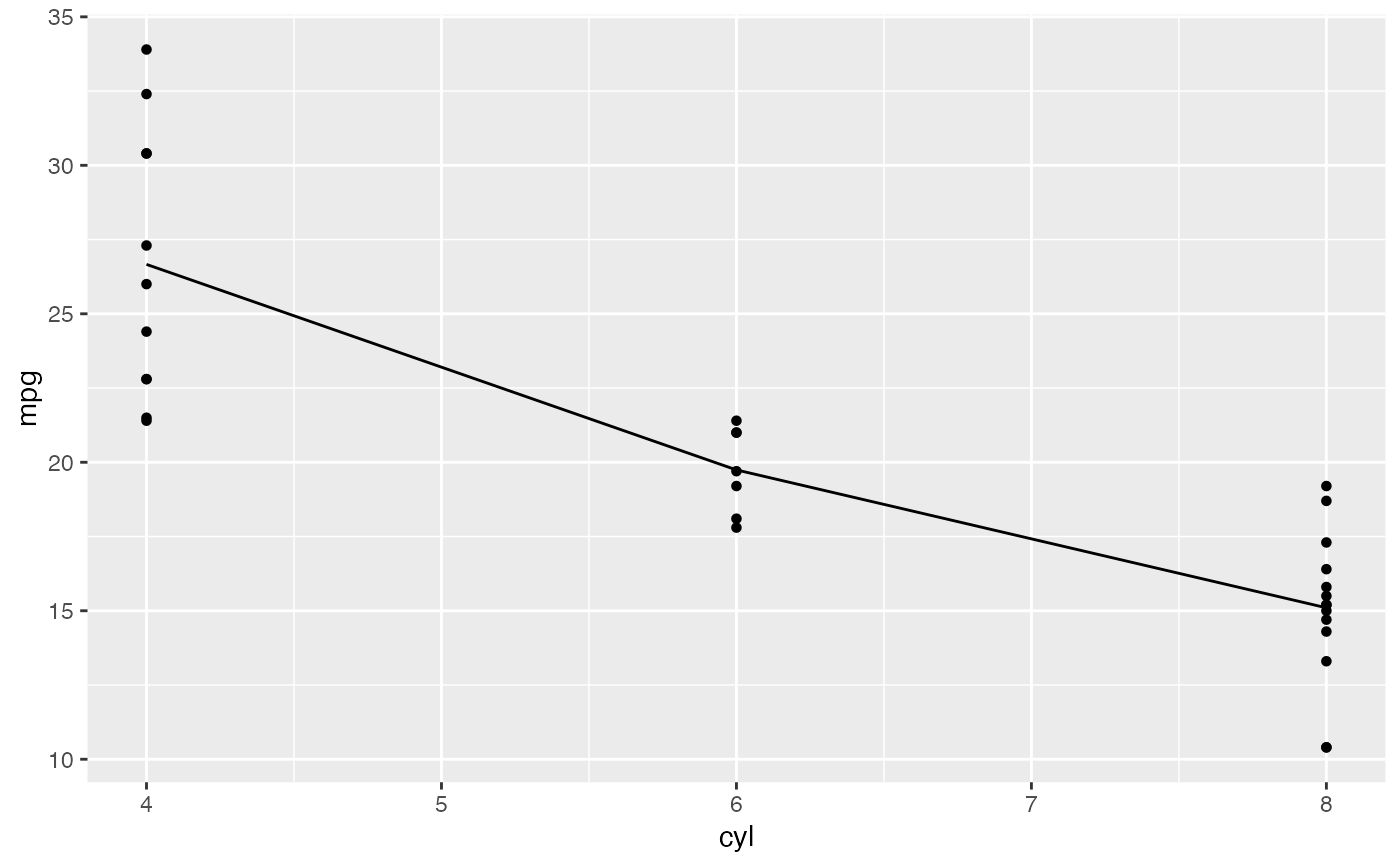
mod <- lm( mpg ~ factor(cyl), data = mtcars)
plotModel(mod)


# SLR
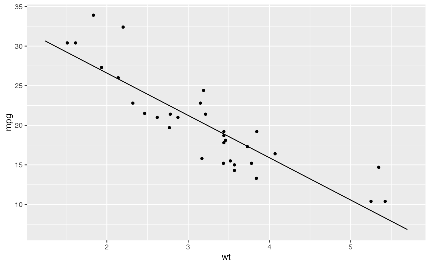
mod <- lm( mpg ~ wt, data = mtcars)
plotModel(mod, pch = 19)


# parallel slopes
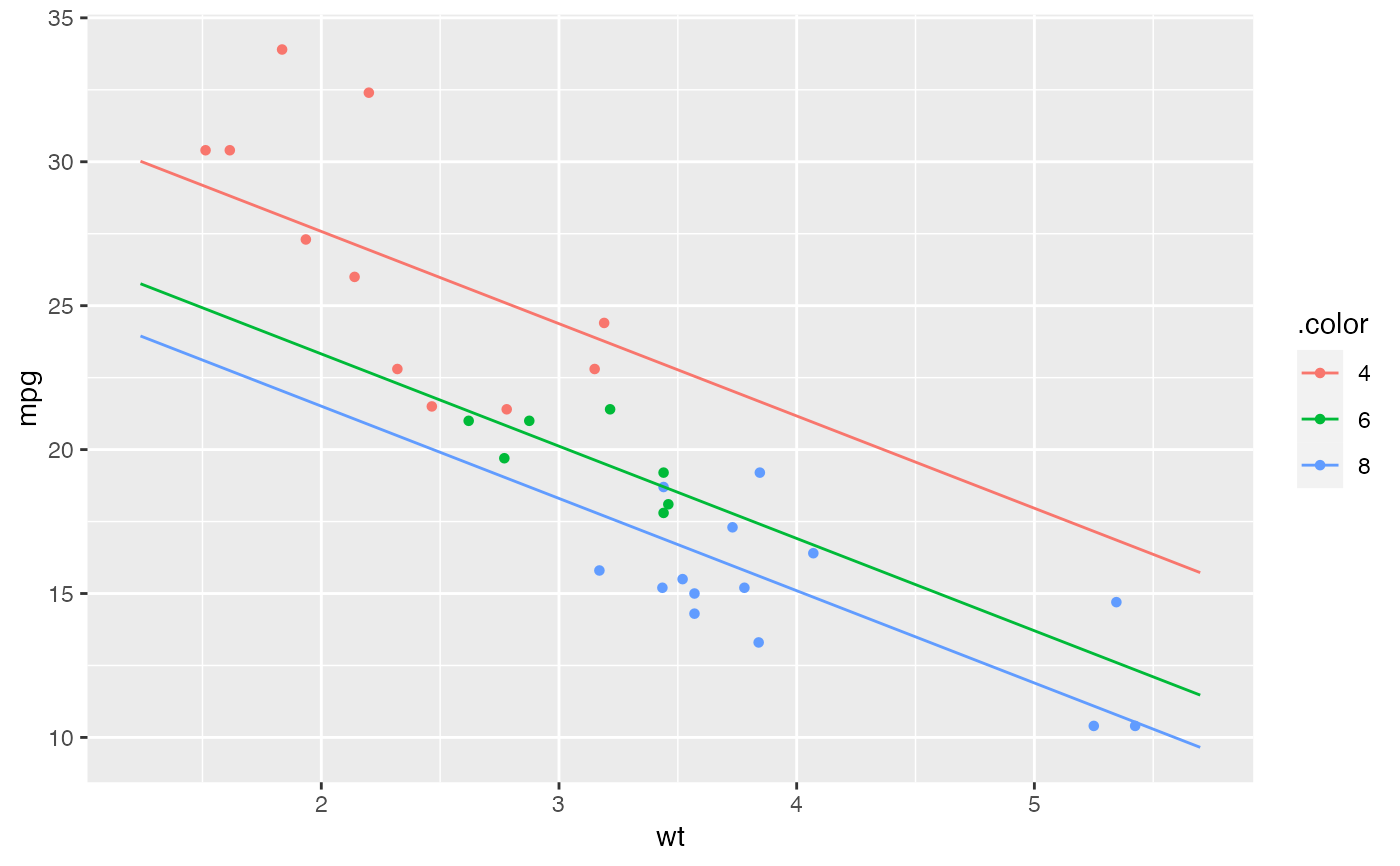
mod <- lm( mpg ~ wt + factor(cyl), data=mtcars)
plotModel(mod)


if (FALSE) { 
# multiple categorical vars
mod <- lm( mpg ~ wt + factor(cyl) + factor(vs) + factor(am), data = mtcars)
plotModel(mod)
plotModel(mod, mpg ~ am)

# interaction
mod <- lm( mpg ~ wt + factor(cyl) + wt:factor(cyl), data = mtcars)
plotModel(mod)

# polynomial terms
mod <- lm( mpg ~ wt + I(wt^2), data = mtcars)
plotModel(mod)

# GLM
mod <- glm(vs ~ wt, data=mtcars, family = 'binomial')
plotModel(mod)

# GLM with interaction
mod <- glm(vs ~ wt + factor(cyl), data=mtcars, family = 'binomial')
plotModel(mod)
# 3D model
mod <- lm( mpg ~ wt + hp, data = mtcars)
plotModel(mod)

# parallel planes
mod <- lm( mpg ~ wt + hp + factor(cyl) + factor(vs), data = mtcars)
plotModel(mod)

# interaction planes
mod <- lm( mpg ~ wt + hp + wt * factor(cyl), data = mtcars)
plotModel(mod)
plotModel(mod, system="g") + facet_wrap( ~ cyl )
}